Spatial dependencies in land use and irrigation access in Northern Peru

Spatial relations are explicitly modelled using spatial weighting matrices which can be applied to the dependent, independent or error terms in regressions

Eduardo Zegarra Group for the Analysis of Development (GRADE), Lima, Perú

Abstract

The potential existence of spatial dependencies in land use and irrigation access in mountainous areas like the Peruvian Andes is a relevant issue for designing and implementing more effective policies for landscape management. In this paper we explore some of these potential interactions in the northern Andean region of Cajamarca (Peru) using a “spatial econometrics” approach. Spatial relations are explicitly modelled using spatial weighting matrices which can be applied to the dependent, independent or error terms in regressions. We estimate alternative specifications of spatial models assessing their statistical robustness. We find evidence of the importance of upstream land use decisions for increasing irrigation access.

Introduction

In this study we evaluate factors shaping access to irrigation in the northern region of Cajamarca, one of the most agrarian (and poorest) areas of Peru. The potential for developing more irrigation in the Peruvian Andes is a key issue in the ongoing discussion about possibilities for eradicating poverty in the most deprived regions of the country. In this work we find evidence on the importance of geographical, institutional, and some farmers”™ attributes influencing irrigation access, and these should be taken into account to make policy more effective and sustainable over time.

In particular, we are interested in finding evidence about the potential existence of spatial dependencies in land use and irrigation access in mountainous areas like the Peruvian Andes. This issue is key for designing and implementing effective irrigation policies and landscape planning strategies. With land and water use ranging from 0 to 4,000 meters above sea level (m.a.s.l) within the same Andean basin, the possibility of multiple spatial and social dependencies becomes a key factor for understanding and assessing options and policies for expanding irrigation access, a key factor for increasing agricultural productivity and income. Access to irrigation is a topic in which these interactions may be especially important in the Andean context as water is stored (naturally or artificially) in upstream snowy peaks (nevados), ponds, lakes or dams, and must travel downstream through a set of rivers, tributaries and channels to reach a myriad of (mostly clustered) irrigators.

In this study we explore some of these interactions in the northern Andean region of Cajamarca (Peru) using a “spatial econometrics” approach. Spatial relations are explicitly modelled using spatial weights matrices which can be applied to the dependent, independent or error terms in regressions. To our knowledge, there has not been previous applications of this approach to the Andean environment, which offers a promising venue for improving knowledge and policy options for land and water management (Lewis et al, 2008).

Our study fits into an increasing amount of research using a geographical or spatial analysis to assess irrigation access around the world. For instance, Lozano-Espitia and Ramirez-Villegas (2016) use geo-referenced information at municipality level in Colombia to assess the impacts of various rural infrastructures (including irrigation) in the productivity of crops. Lobell et al (2010) use satellite data for identifying factors affecting yields in India, finding that the distance to irrigation canals has statistically significant impacts on increasing crop yields.

Literature review

There are thousand of entries in the international literature regarding irrigation and its role in economic and social development. For the purposes of this study, we distinguish some approaches that seem to us are most useful. First, there are many studies assessing the impact of irrigation on various measures of well-being, asset value and productivity of farmers. Joshi et al (2017) estimated an increase of 46% in the value of the land associated with the irrigation versus those that do not have this status in Nepal. Dillon (2011) estimated that access to irrigation increases the consumption of households in 27-30% in rural Mali, with increases in the accumulation of livestock assets as well. For Ethiopia, Gebregziabher et al (2009) calcalated an impact of more than 50% in farmers”™ income from irrigation, whereas Yasuyuki et al (2014) show for Sri Lanka that access to irrigation not only raises incomes, but also changes the flows of these, reducing the likelihood of being credit constrained in financial markets. For Peru, using the National Household Survey-ENAHO, Zegarra (2014) found significant impacts on the incomes of farmers in the three natural regions. For the coast, the expected income impact is 1,584 annual soles per capita; in the sierra of 593 soles and in the jungle of 1,267 annual soles per capita. In all these studies, focusing on impacts on income, consumption or some assets, the evaluation is done at the level of agricultural households, usually with comparison to control groups. In these cases, it less common to find geographic variables playing some role as critical determinants for access or impacts of irrigation.

A related entry of interest are the ones analyzing diverse factors that determine access to irrigation, both at the level of individual farmers and at different levels of social or geographic aggregation. It should be noted that some of the previous studies that assess impacts, also perform some micro-economic analysis of factors that determine individual access. This analysis is needed to establish the comparability between the treatment and control groups. An example of this type of analysis is Sinyolo et al (2014) for South Africa. The authors find statistical relevance for factors influencing irrigation access in variables like perceived fertility of the soil, size of households and access to support services, that they consider as good predictors of access to irrigation in a sample of farmers.

There is another set of works that take a more geographical or spatial approach both for the estimation of impacts and, sometimes also for identifying factors influencing irrigation, which is the approach that we adopt in the present study. For instance, Lozano-Espitia and Ramirez-Villegas (2016) use georeferenced information at municipality level in Colombia to assess the impacts of various rural infrastructures (including irrigation) in the productivity of crops. Lobell et al (2010) use satellite data for identifying factors affecting yields in India, finding that the distance to irrigation canals has statistically significant impacts on increasing crop yields.

There are also studies relating climate change and irrigation in different contexts. Causality in these studies may go from the effects of climate change to the patterns and practices of irrigation (Ponce et al, 2015; Zhang et al, 2015; Skarbo and VanderMolen, 2014), or from irrigation adoption and practices into climatic variables and their interaction with the process of climate change (Im et al, 2014; Okada, 2015).

Another line of work (of most interest to us) is the assessment of various geographical, economic and institutional variables to estimate and predict access to irrigation. A still small branch of research is related to institutional factors (such as communal organization, levels and types of land tenure) in access to irrigation. A study of this type is Saldias et al (2013) for Bolivia, who assess the variability in access to irrigation for various forms of community organization in a large rural area of Bolivia. A more qualitative analysis was carried out for the Sierra Colca Valley (Arequipa) in Peru by Delgado and Linden (2013).

A related branch of research seeks to estimate the potentials for irrigation development in particular geographical contexts. You et al (2014), for example, use geographic models to identify areas with the greatest potential for the development of irrigation in Kenya. A previous work of this type (You et al, 2011) generated estimates for the entire African continent, based on a composition of different layers with geographical information on water availability, topography, expected yields and existing and planned water storage capacity. A similar exercise for Ethiopia is the one of Worqlul et al (2015); and the development of irrigation with groundwater from Ghorbani et al (2017) in Iran.

A general trait of these studies is that, even as these are geographical, the spatial interactions of observational units are not explicitly modelled. This is what distinguishes the so called spatial econometric approach (Anselin, 2003; Kelejian and Piras, 2017). In this approach spatial dependencies are explicitly modelled using weighting matrices with some associated parameters that account for the strength of the spatial dependency. A critical advantage of this modelling (over standard non spatial linear regressions) is that spatial autocorrelation (for example in errors) is generally reduced or eliminated, rendering more consistent estimates of coefficients.

Area of study and data description

The northern Peruvian region of Cajamarca (limiting with Ecuador) may be considered as the most agrarian region in the country: it has the largest number of farmers, 340,000 or 16% of total according to the last agricultural census (CENAGRO, INEI, 2012). It is also one of the poorest regions, with very high incidence of poverty and extreme poverty. The agricultural sector is characterized by severe difficulties for farmers to accessing infrastructure, markets and services (Zegarra and Calvelo, 2006).

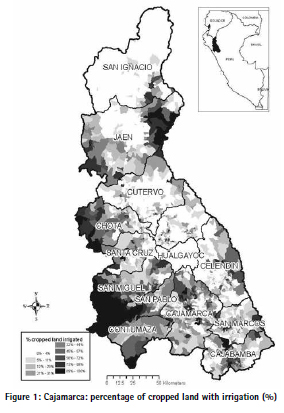
In terms of irrigated land, Cajamarca ranks 13 of 20 among sierra regions, with 66,000 Ha. of irrigated land, representing 21% of cropped agricultural area. The per capita area under irrigation of Cajamarca is only 0.289 Ha per farmer, well below some of the most important regions of Sierra. The average allocation of area under irrigation in Cajamarca can hide important variations within the region, as can be seen in Figure 1 with the location of census tracts and their percentage of cropped land under irrigation.

Access to irrigation is heterogeneous across the region, with more relative access in the lower western areas of San Miguel, San Pablo, Chota and Jaén and in the eastern areas of Jaén and in less extent Celendín. The southern side of Cajamarca province and central parts of Cajabamba also show more relative access to irrigation.

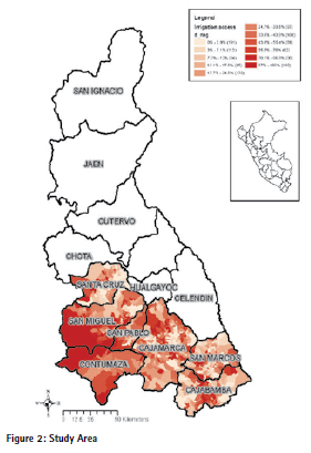
Some provinces like San Ignacio, Cutervo, Hualgayoc and most of eastern Chota do not have irrigation at all. For this study we focus on seven southern provinces of the region as shown in Figure 2 which also displays the percentage of agricultural land under irrigation in each agricultural census tract.

Access to irrigation is heterogeneous across the study area, with more access in the low altitude coastal zones. Table 1 shows means (by agricultural tract) of geographical, climate, land use and socio-economic variables. Mean values are measured across quintiles according to the proportion of cropped area under irrigation. As basic geographical variables1 we include altitude, slope and the shortest Euclidean distances from census tracts”™ centre points to water sources like rivers and dams (excluding dams related to mining). As rainfall and temperature variables we projected data from meteorological stations to the overall study area. These variables are potentially important in influencing both the water supply and the demand for irrigation. From the 2012 agricultural census we calculated land use (forest, pasture and permanent crops) and other socio-economic variables like number of farmers, percentage without land title, age and education that are factors potentially affecting irrigation patterns as well. We also estimated Euclidean distances to the nearest city (of more than 3,000 inhabitants) to account for distance to market.

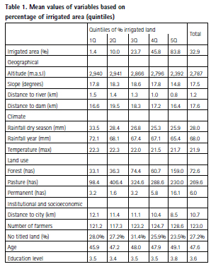
Descriptive figures in Table 1 show some potential patterns along irrigation quintiles. Less irrigation is more likely to occur with higher altitude, and longer distances to rivers and to dams, and also with steeper slopes and more rainfall (both yearly and in the dry season). Relationships of irrigation with land use variables like presence of forest and permanent crops appear to be positive whereas the relationship with pastures is ambiguous. More distance to markets appears to be negatively related to irrigation, whereas lack of land title may also influence irrigation. Finally, some variables directly related to farmers as age and educational attainment were considered. Apparently, there is a positive relationship between age and education with more irrigation access.

While this initial analysis suggests some potential relationships, it is necessary to evaluate the whole set of explanatory variables using a more formal model and a regression framework that will allow us to establish relationships in a more comprehensive manner, taking into account potential causalities and spatial dependencies. This is what we present in the following section.

Modelling access to irrigation with geographic models

The literature review that was presented earlier summarized different approaches to the quantitative analysis of irrigation under separate socio-economic and geographic contexts. The existence of irrigation will depend not only on geographical factors –  such as topography, type of soil, availability of water, precipitation, and distance to alternative sources – but also on several socio-economic and institutional conditions, including public investment, institutional and organizational capacity, and access by the various actors to resources. For this work our goal is to combine these elements into one coherent analytical model that includes with the greatest possible precision some of these geographical and socio-economic factors. Naturally, we proceed cautiously because of the possibility that these ‘measurable’ empirical variables may not represent adequately or appropriately the theoretical variables.

The most important consideration is the exogeneity of the explanatory variables, and their orthogonality relative to the corresponding error terms. Nevertheless, equally important in models incorporating geographical variables, is the basic assumption about the area or unit of analysis, which in our case will be the agricultural census tracts. It is assumed that our level of analysis is sufficiently detailed to permit the identification of relevant spatial patterns that can explain the phenomenon of interest, namely the extension of irrigation in this territory. With these assumptions we can produce consistent estimates, and – at the same time – generate predictions about the level of irrigation that could exist in the conglomerates, according to the structural conditions, as functions of the independent variables.

Thus, historic, geographic and institutional factors influence irrigation location and expansion. Feasibility of irrigation depends on the topography, soil type, availability of water, distance to alternate water sources, but also on socio-economic and institutional factors like past public investment, institutional capacity and social organization, available resources, among others (Kang, 2017; Tsukasa et al, 2013). A key point is that irrigation tends to locate in specific sites, forming clusters. This is expected as irrigation infrastructure shows economies of scale: it is more efficient to build one large integrated irrigation system (reservoirs and canal networks) in one location than many small and dispersed units in a given basin (Zegarra, 2002).

Given these specific features, we need to model access to irrigation as a combination of geographic, climate, land use and socio-economic factors that would reflect- -as accurately as possible–some of these characteristics in a particular landscape. For this we consider a very general spatial model like the one described by Kelejian and Piras (2017) for N observations (census tracts):

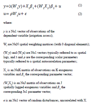
Matrices W’s are very important for the explicit spatial specification of the model as these will represent the expected degree of interaction between any observations and neighboring (or more or less closer) units in the same territory. The values (weights) in these matrices try to represent spatial interactions among observations, and parameters ג, 𝜌 and 𝛽2 measure the direction and intensity of these interactions. In terms of an econometric specification, when when ג and 𝜌 are assumed equal to 0, the model is the traditional non spatial Ordinary Least Square (OLS). If the “true” model has strong spatial autocorrelation, an OLS estimation of (1)-(2) will generate inconsistent estimates of parameters given the endogeneity of the autoregressive term (Drucker et al, 2013).

The matrix (W2X2) and vector of parameters 𝛽2 are also important to account for specific spatial dependencies among some specific exogenous variables and the dependent variable. In particular, in our case we will use 𝛽2 the coefficients to estimate the expected effect of exogenous land use variables in the upstream areas on the endogenous irrigation access.

Spatial weights matrices

As discussed in the previous section, a key element in any spatial modelling is the spatial weighting matrix that will identify spatial interactions. How these matrices are specified and used is a central tenet of spatial modelling. In the spatial weighting matrix we define which units are spatially interacting and the intensity of such interaction. It is generally assumed that closer units will have a stronger interaction with a given unit. In summary, the spatial matrix will define which units interact (are considered “neighbours”) and what weight will be given to its “influence” on the observed unit (generally depending on distance).

In our case we have two types of weighting matrices in our modelling. First there are the W1 and W3 type of matrices as shown in expression (1) which are used for spatially lagging the dependent variable and/or the error term, respectively. For these matrices we generated the standard weighting matrix (W=W1=W3) based on distance, with a distance decay function for neighbours of up to 20 Km distance from each census tract. This is the matrix we will use for different specifications of (1)-(2).

But we also considered a spatial matrix for lagging some of the independent variables (W2 type of matrix). This is particularly important for modelling spatial interactions in which we expect that some of the independent variables will have a certain type of spatial relationship with the dependent variable. In the case of irrigation, the ideal data for modelling spatial interactions would be detailed network data, i.e., to know what units are connected along the irrigation networks. However, this type of data is not easily available, especially for large areas as the one we want to model. Instead, we propose as a feasible option to use the altitude variable for restricting the spatial weighting matrix in order to better reflect the relationship between irrigated and upstream areas in the Andean context.

To operationalize this idea we order the census tracts according to increasing altitude. After doing this we can impose the constraint that no neighbouring unit (within a given distance) can have a lower altitude than the reference unit. This is equivalent to defining that only upstream units are considered as neighbours to each observation.

Thus, we can think of two types of matrices for the study area. The first type of matrix is the normal circle around each observation that can be considered “symmetric” in terms of altitude (W=W1=W3). The neighbours of a given unit may be at higher or lower altitude, and being a neighbour only depends on Euclidean distances to the observed unit (in a circular area of influence). The second type of matrix (W2) is asymmetric in terms of altitude as we impose the restriction that a neighbour for a given unit can only be located at higher altitude within a given distance. A graphic comparison of both types of matrices can be seen in the figure 3.

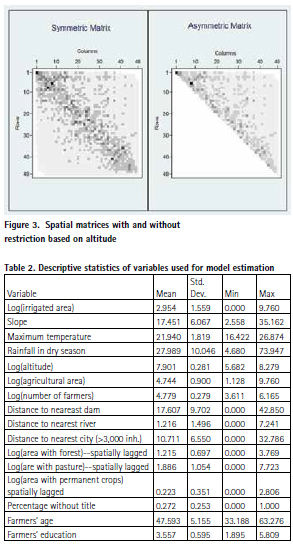
Notice that in the restricted version there are no neighbours below the matrix’s diagonal, as these are located at a lower altitude (neighbours can only be located at a higher altitude). We apply the W2 spatial lagging matrix to the land use variables we think may influence access to irrigation in the downstream areas: area if land with forest, pasture and/ or permanent crops. These are the only exogenous variables which will be spatially lagged in our estimations.

Estimating alternative specifications

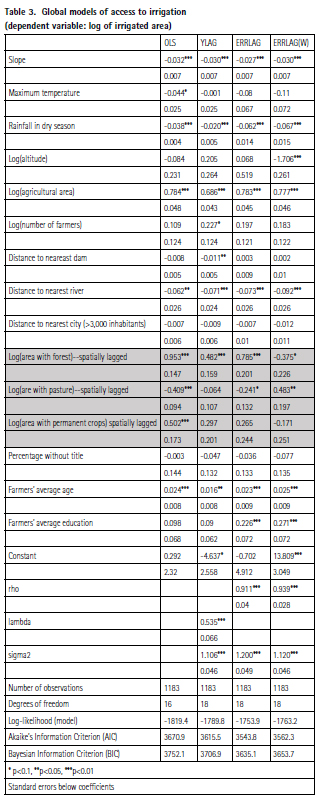
We will use as dependent variable the log of irrigated area in each census tract. For some of the continuous X variables we also adopted logarithmic transformations2. The descriptive statistics and units of measurement of the variables used for estimating the models3 is presented in Table 2. We include the log of total agricultural land per tract as an independent variable in order to control for any spurious scale effect coming from using as dependent variable the (log of) total irrigated land per tract.

We estimate three specifications of the global model: (i) non spatial OLS, assuming no spatial autocorrelation (ג and 𝜌 are equal to 0); (ii) LAGY, spatial correlation only in the dependent variable 𝜌 =0, known as SAR model, and (iii) LAGERR, spatial correlation only in the error terms so ג =0. We also include a fourth column (iv) in which the LAGERRR model is run with the symmetric W matrix for lagging the land use variables (to check if the choice of W is important). The results are presented in Table 3.

An important issue is how to select the best specification given the data we used for the estimation. In this case the literature recommends using the information criteria such as the Akaike Information Criteria (AIC) and Schwarz’s Bayesian Information (BIC). The specification with the lowest value for these criteria is considered the best specification. In this case, the LAGERR specification has the lowest values in both criteria so it is the best specification we can get from these alternative spatial models. We also tried the model selection criteria proposed by Anselin (2005) based on Lagrange Multiplier tests where the OLS specification is compared to alternative spatial models. Using the robust version of the tests as suggested by Anselin4 we find that only the error lag model is statistically significant and is indeed the best of the three alternative specifications for these data.

Most geographic variables have significant coefficients and expected signs in all the specifications. Altitude and slope have negative impacts on irrigated land as well as distance to rivers, as expected. Less rainfall in the dry season is important in explaining more irrigation (so this can be interpreted as a crop demand effect). Mean rainfall for the whole year, however, appears as no significant as well as maximum temperature. These results may be related to the limited spatial variability of these variables after smoothing the data with geographic interpolation algorithms based on few meteorological stations (10 for temperature, 13 for rainfall).

In the land use variables, the area with forest is positively associated with irrigation whereas the one with pasture decreases irrigation access. This can be expected as more forest tends to generate better conditions (less erosion) for water regulation in the upper parts of Andean basins, whereas more pasture (linked to more cattle) will have the opposite effect.

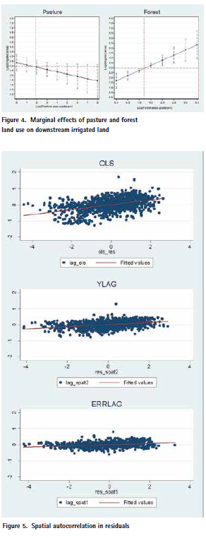
Given that the dependent and independent variables are in logs, the coefficients can be interpreted as elasticities. The value of the irrigated land to forest elasticity is 0.785, and for pasture is -0.241. This implies that an increment of 10% in forest land in the upper parts of the basins will increase irrigated land in 7.8%. In the case of pasture, an increase of 10% in land devoted to this use will reduce irrigated land by 2.4%. These are important effects and are plotted in Figure 4 for alternative values of the covariates. The mean of the dependent and each independent variable are also shown in the figure 4.

Also notice that in the fourth column of Table 3 – where the spatial lagging of land use variables is based on a symmetric W2 that does not considers altitude for choosing neighbors – the signs of these two coefficients are reversed and potentially misleading. This is an indirect proof of the importance of a correct specification of W2 in order to capture the spatial dependencies in this context.

In terms of socio-economic variables, age and education appear with positive and significant coefficients in the (preferred) error lag specification. Life cycle and human capital considerations seems to be important for this result. Note that the education effect is not picked up neither by the OLS or YLAG models.

The estimated spatial coefficients ρ and λ are significant in both spatial specifications indicating that global spatial dependencies modelled with the spatial weight matrices are important explanatory factors. The estimated error lag coefficient is 0.91, indicating strong spatial autocorrelation in the data. The high value and significance of this spatial autocorrelation parameter indicate that the OLS estimates are very likely to be inconsistent.

In Figure 5 we present Moran’s scatter diagrams of estimated residuals (versus spatially lagged residuals using the same 20 Km weight matrix) for the first three specifications.

In Table 4 we report the estimated Moran”™s I coefficients for each model.

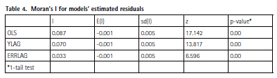
From the table and the graph we see that ERRLAG is the most effective in reducing the strong spatial autocorrelation found in the global OLS. However, notice that the Moran I”™s coefficient is statistically significant for the ERRLAG, so some spatial autocorrelation in residuals still remains even with these explicit spatial specifications.

Conclusion

In this study we estimate spatial models for irrigated land in Northern Andes of Peru considering geographic, climate and socio-economic factors. Most geographic variables show significant coefficients an d expected signs. Higher altitudes and steeper slopes have negative impacts on irrigated land as well as distance to rivers. In the climate variables, less rainfall in the dry season is important in explaining more irrigation and this can be interpreted as a demand effect. Neither mean rainfall for the whole year nor maximum temperature appear to be important for explaining irrigated land in this context.

We also find strong statistical evidence that land use practices (forest and pasture) in the upper areas of Andean basins have high influence in explaining irrigation in the lower zones of the same basin. The irrigated land to forest elasticity is almost 0.8 and for pasture is -0.24 (although less precise), which are important magnitudes. This finding suggests that promoting the adoption of more forest (trees) in the upper basins will be really effective for facilitating or/and ensuring more irrigation downstream. Also, it is clear that more cattle and pastures in the upper highlands of Cajamarca will have a negative effect on irrigation in the lowlands. Both findings will also support potential benefits coming from implementing mechanisms of payments for ecosystem services, for instance between irrigation organizations and upper land communities. These schemes are only viable with the participation of local and national authorities and with clear normative instruments and incentives for both parties

Our study also has some contributions in terms of methodology. We find that a correct specification of the spatial weighting matrix for lagging the land use variables is crucial for getting correct results in a context where we do not have detailed information on the shape and real water interactions within irrigation networks like spatial dependencies. However, in the Andean context we were able to correctly detect and estimate some of these spatial relationships using the altitude variable for constraining the weighting spatial matrix. Finally. we also found for these data and context that the error lag model is the best spatial specification for the estimations, obviously better than the non spatial OLS but also than the autoregressive dependent variable specification.

End notes

¹All geographic and climate data for this research were processed and analysed with © ESRI ArcMap 10.1.

²For any “x” that is log transformed we used ln(x+1) to avoid the occurrence of missing values when x is zero.

³For the econometric estimation of (1)- (2) we use © Stata, version 13.0, with its module for estimating spatial regressions with the maximum likelihood option. The software allows users to build matrices W and M based on spatial data.

⁴For carrying these tests we used GeoDaTM, a software developed by Luc Anselin, version 1.14.0 updated August 24, 2019.

⁵It should be noticed that the Moran”™s I may be also picking heteroskedasticy in error term as pointed out by Anselin (2005)

References

Anselin Luc, 2003. Spatial Externalities, Spatial Multipliers, and Spatial Econometrics. International Regional Science Review. 26,2,153166

Anselin Luc, 2005. Exporing Spatial Data with GeoDa: A Workbook. Center for Spatially Integrated Social Science. University of Illinois, Urbana-Champaign. Revised Vesion. March 6, 2005. 225 pp.

Delgado, Juana Vera Vincent, Linden (2013) “Community irrigation supplies and regional water transfers in the Colca Valley, Peru.” In Mountain Research and Development. Vol. 33.

Dillon, Andrew (2011) “The Effect of Irrigation on Poverty Reduction, Asset Accumulation, and Informal Insurance: Evidence from Northern Mali” in World Development. Vol. 39.

Drucker D., I. Prucha and R. Raciborski, 2013. Maximum likelihood and generalized spatial two-stage leastsquares estimators for a spatialautoregressive model with spatialautoregressive disturbances. The Stata Journal. 13, 221-241.

Georganos S., A. Abdi, D. Tenenbaum and S. Kalogirou, 2017. Examining the NVDI-rainfall relationship in the semi-arid Sahel using geographically weighted regression. Journal of Arid Environments, http://dx.doi. org/19.1016/j.jaridenv.2017.06.004.

Ghorbani Nejad, Samira, Fatemeh Falah, Mania Daneshfar, Ali Haghizadeh, and Omid Rahmati, 2017. Delineation of groundwater potential zones using remote sensing and GISbased data-driven models. Geocarto International. 32, 2, 167-187.

Gebregziabher, Gebrehaweria Namara, Regassa E. Holden, Stein (2009) “Poverty reduction with irrigation investment: An empirical case study from Tigray, Ethiopia” in Agricultural Water Management. Vol. 96

Im Eun-Soon Marcella, Marc P. Eltahir, Elfatih A. B., 2014. Impact of Potential large-scale Irrigation on the West African Monsoon and Its Dependence on Irrigated Area of Location. The Journal of Climate. 27,3, 994-1009

INEI: Instituto Nacional de Estadística e Informática, 2012. IV Censo Nacional Agropecuario. Resultados Preliminares. Lima, December 2012. 93 pp.

Kang Dongwoo, 2017. Essays on Spatial Externality and Spatial Heteregeneity in Applied Spatial Econometrics. PhD Dissertation. The University of Arizona.

Kelejian Harry and Gianfranco Piras, 2017. Spatial Econometrics. Academic Press, Elsevier. Cambridge, MA, USA, 2017

Leng Guoyong, Tang Qiuhong, 2014. Modeling the Impacts of Future Climate Change on Irrigation over China: Sensitivity to Adjusted Projections. Journal of Hydrometeorology. 15,5,2085-2103

Lewis David, Bradford Barham, Karl Zimmerer, 2008. Spatial Externalities in Agriculture: Empirical Analysis, Statistical Identification and Policy Implications. World Development. 36, 10, 1813-1829

Lobell D., J.I. Ortiz-Monasterio, A.S. Lee, 2010. Satellite evidence for yield growth opportunities in Northwest India. Field Crops Research. 118, 1, 13-20.

Lozano-Espitia Ignacio and Lina Ma. Ramirez-Villegas, 2016. How Productive is Rural Infrastructure? Evidence on Some Agricultural Crops in Colombia. Borradores de Economia 948, 2-20.

Nakaya T., M.n Charlton, C. Brunsdon, P. Lewis, J. Yao, A. S. Fotheringham, 2009. GWR4 Windows Application for Geographically Weighted Regression Modelling. User Manual.

Neumann K., E Stehfest, p. Verburg; S Sibert; C. Müller; T Veldkamp, 2011. Exploring global irrigation patterns: a multilevel modelling approach. Agricultural Systems 104,703-713.

Okada, Masashi Iizumi, Toshichika Sakurai, gene Hanasaki Naota Sakai, Toru Okamoto, Katsuo Yokozawa, Masayuki, 2015. Modeling irrigationbased climate change adaptation in agriculture: Model development and evaluation in Northeast China. Journal of Advances in Modeling Earth Systems. 7,3,1409-1424.

Ponce Carmen, Carlos Alberto Arnillas, and Javier Escobal, 2015. Cambio climático, uso de riego y estrategias de diversificación de cultivos en la sierra peruana. Chapter in Escobal J., R. Fort, and E. Zegarra (Eds.), 2015. Agricultura peruana: nuevas miradas desde el Censo Agropecuario. Lima: GRADE.

Saldias, Cecilia Speelman, Stijn Van Huylenbroeck, Guido (2013) “Access to Irrigation Water and Distribution of Water Rights in the fan of Punata, Bolivia.” In Society & Natural Resources. Vol. 26

Shi Shu qin; Cao Qi-wen, Yao Yanmin, Tang Hua-jun, Yang Peng, Wu Wen-bin, Xu Heng-zhou, Liu Jia and Li Zheng-guo, 2014. Influence of Climate and Socio-Economic Factors on the Spatio-Temporal Variability of Soil Organic Matter: A Case Study of Central Hellongjiang Province, China. Journal of Integrative Agriculture. 13,7, 1486-1500.

Sinyolo, Sikhulumile Mudhara, Maxwell Wale, Edilegnaw (2014) “The impact of smallholder irrigation on household welfare: The case of Tugela Ferry irrigation scheme in KwaZulu- Natal, South Africa”. Water SA. Vol. 40 Tsusaka T akuji, Kei Kajiza, Valerien Pede and Keitaro Aoyagi, 2013. Neighborhood effects and social behavior: the case of irrigated and rainfed farmers in Bohol. The Philippines. MPRA Paper N° 50162.

Worqlul, Abeyou W., Amy S. Collick, David G. Rossiter, Simon Langan, and Tammo S. Steenhuis, 2015. Assessment of surface water irrigation potential in the Ethiopian highlands: The Lake Tana Basin. Catena. 129, 76-85.

Yasuyuki Sawada Masahiro Shoji Shinya Sugawara Naoko Shinkai (2014) “The Role of Infrastructure in Mitigating Poverty Dynamics: The Case of an Irrigation Project in Sri Lanka.” B.E. Journal of Economic Analysis & Policy. Vol. 14.

You, Liangzhi, Ringler, Claudia Wood- Sichra, Ulrike Robertson, Richard Wood, Stanley Zhu, Tingju Nelson, Gerald Guo, Zhe Sun, Yan, 2011. What is the irrigation potential for Africa? A combined biophysical and socioeconomic approach. Food Policy. Vol. 36.

You, Liangzhi Xie, H. Wood-Sichra, U. Guo, Z. Wang, Lina, 2014. Irrigation potential and investment return in Kenya. Food Policy. 36,6,770-782.

Zegarra Eduardo, 2002. Water Market and Coordination Failures: The Case of the Limari Valley in Chile. PhD Dissertation. University of Wisconsin- -Madison, 2002 – 138 pp.

Zegarra Eduardo and Daniel Calvelo (2006). “Cajamarca: Lineamientos para una política regional de agricultura”. En Contribuciones para una visión del desarrollo de Cajamarca. Francisco Guerra-García (eds). Volumen 4. Asociación Los Andes de Cajamarca. Cajamarca, Peru.

Zhang Tianyi Lin, Danny Rogers and Freddie Lamm, 2015. Adaptation of Irrigation Infrastructure on Irrigation Demands under Future Drought in the United States. Earth Interactions. 19, 7,1-16.

Zhao Gang Webber, Heidi Hoffmann, Holger Wolf, Joost Siebert, Frank Ewert, 2015. The implication of irrigation in climate change impact assessment: a European-wide study. Global Change Biology. 21, 11, 4031-4049.

The paper prepared for presentation at the”2020 World Bank Conference on Land and Poverty” The World Bank – Washington DC, March 16-20, 2020. Copyright 2020 by author(s).