| GIS | |
The use of GIS to forecast tourism demand
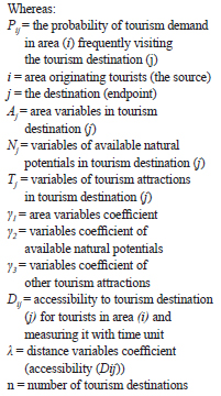
Most applied methods to determine the tourism demand depend on the availability of demographic data, social and economic characteristics of tourists, tourism customs, the quality of tourist activities and facilities, and other foundations such as the capacity of the tourist destination, and its accessibility. So, a tourism site must be designed in accordance with the standards and regulations of great importance in the protection of environment resources, and to develop appropriate plans to meet the expected demand for tourism. The urban planning optimal tourism sites take into account the number of tourists forecast, whenever available accurate data on flow of tourists in the area, which makes tourism development more accurate and logical Because such information can often be unavailable or inadequate to forecast tourist numbers; due to lack of monitoring mechanisms set up, tourists and limitations add to the cost and effort and duration (Ghoneim, 2003). Define and analyze trade areas help forecast tourism flows. The study goals to achieve the following: 1. Develop an approach for forecasting tourism demand by GIS. 2. Identify the different factors and variables that play an important role of spatial interaction related to tourism demand. 3. Design the necessary database for the model using GIS for a site with real data (Al-Uqair). 4. Implement the automated model, checking its validation, and discussing the possibility of generations. 5. Determine the geographic distribution pattern of the model output and discussing it in the light of the pros and cons of the automated application of the model. This study uses (ArcGIS Business Analyst), since these systems are designed to analyze and interpret spatially, in addition to calibrating the Huff model to measure tourist numbers through a real case study (Al-Uqair). There are several reasons behind the selection of Huff model in this study. First, the form is theoretically attractive; as the logical underpinning of the model makes sense and the output can be communicated easily and understandably. Secondly, the model is relatively easy to make operational. The necessary computations are straightforward once the values of the variables and parameters are specified. The third reason for the model’s popularity is its applicability to a wide range of problems and its ability to predict outcomes that would be difficult, if at all possible, without the model. Despite the general applicability of the model, it has not always been employed correctly. Furthermore, the full potential of the model has not been realized. Study backgroundDavid Huff introduced his model in 1964, which takes into account the number of consumers, the attractiveness of business centers, and the distance and competing commercial centers that predict consumer behavior spatially. Huff model is derived from the theories which are based on spatial analysis which are based on the principle that the prospect of a buying or visiting consumer to a particular site depends on the distance and the attractiveness of the site and the distance and attractiveness of competing sites. This model is used in spatial interactions researches (Huff, 1964). Trade areas analysis models provide great potential for the formulation and appraisal of geographic business decisions. The Huff model was widely used by business analysts in the public and private sectors as well as academics across the world. The popularity of the model increased with the development of the GIS technology. For example, the model can be used in the field of trade for the following purposes: Assessing market prospects; identifying and analyzing trade areas; assessing market penetration; estimating the economic impact; forecasting consumer choices in shopping; describing the distribution of consumers geographically, and estimating the sales size for the current and potential selling outlets (Huff, 2008). As the case in the trade field where the commercial market penetration is forecast through geographic scope, the same idea could be used to analyze the potential tourism demand, as a commodity subjected to the supply and demand laws. Using Huff Model for tourism demand estimationThe actual reality theories of tourism demand as indicated in Kafi’s study (2008) are as follows: (1) the number of inbound tourists is directly proportional to the number of residents and the intensity of their movements; (2) the number of inbound tourists is directly proportional to the relative attractiveness of the tourism destination; (3) the number of inbound tourists is inversely proportional to the distance to the destination (accessibility). This takes into account the competition factor, where the distribution of potential tourists to competing destinations is taken into account according to the distance. The attractiveness of each competing destination plays an important role in the distribution of the number of tourists, and the attractiveness of any tourist destination depends mainly on the available attracting factors, such as the prevailing natural environment, the type of services available, and the image of a destination that affect the tourist when choosing alternatives. The number of tourism facilities in any tourist destination is a reflection of the attractiveness of this destination; thus, when the attractiveness increases, the destination’s facilities increase. In other words, it can be said that tourist destinations that have the greatest facilities have the greatest degree of attractiveness. The Huff model includes many factors and variables affecting the tourism demand which are clarified by previous studies to controllable and non-control variables. The controllable variables could be processed by decision-makers, such as advertisement, tourism packages, prices, and provision of tourism services and infrastructure development. The non-control variables are generally beyond control, such as natural tourism potentials, the archaeological and historical factors, population distribution, distance, and competition. Therefore, the application of the Huff model to forecast the tourism demand requires compiling a list of specific factors. The adopted factors in this study are limited to the significant ones such as spatial vicinity, area, and the availability of natural potentials and other tourist attractions, based on the Hudman study (Hudman, 1980). Both factors are a form of data that will feed the model.
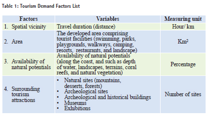
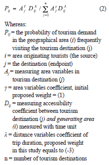
The Huff model is based on the theory that when someone is facing a range of alternatives, the probability of selection is directly proportional to the tangible benefit of that alternative, so the selection behavior is mathematically referred to by (Pij). As a result of the alternative selection process, trips are distributed among different tourism destinations. So, the Huff model will be used to measure the distribution of tourists. The factor of distance traveled by tourists to reach the tourism attractions could be used as a variable. And the distance will be considered a main variable in this study, which is measured by the duration of the trip. Given the importance of the time it takes to travel between the places of residence to the tourist destination, the trip duration gives an overview of the accessibility, the traffic volume, and the status and quality of available roads. The tourist site area reflects the attraction power, i.e., the developed area comprising tourist facilities such as accommodation, resorts, restaurants, parks, landscape, and waterscape related to leisure and entertainment. Table (1) indicates a list of tourist demand factors, variables and measuring units, which will be taken into account in this study for Al-Uqair site and competitive tourist destinations. Spatial vicinity factor is inversely proportional with tourists, while the other factors of area, availability of tourism potentials, and the surrounding attractions are directly proportional to the number of tourists. Mathematical formulation of the Huff Model to forecast tourism demandA phase of analyzing the tourism demand behavior mathematically by linking the effecting factors and variables. It is called ‘the diagnostic since it explains how factors can be linked together through the Huff model. Therefore, the use of the Huff model in this study is as a mathematical equation linking the factors influencing the tourism demand. The Huff model by linking the above mentioned tourism demand factors can be explained by re-explaining the equation number (1) mathematically, as follows:
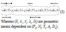
In this stage, the original the Huff model is being calibrated, tested and validated, as the resulting standard model will be used to forecast the tourism demand in the next period. The calibration process of the Huff model’s variables coefficient requires calculating the data of tourism demand probabilities (ratios), its referred to by (Pij) in equation. The calculations of tourism demand probabilities data are based on choosing appropriate initial values – an approximate weights for key variables coefficients (y, n) as a preliminary stage. Therefore, the initial coefficients values are dubious; due to the inability to determine the statistical significance of the variables. The main two variables (distance, area) influencing tourism demand directly can be identified as follows: First: The area represents the tourism attraction variable (Aj). And in the beginning, a coefficient value was proposed (y), which is (1), as neutral value. Second: The distance represents the tourism direct variable (Dij), the distance between the tourist’s place of residence (i) and destination (j). The value of the distance variables coefficient (y) ranges between (-1) to (- 3) by recommendations from the Huff model (Huff, 2008). (-3) will be used in this study; considering that tourism tours are not services that people need every day. In this case, Huff model equation is represented as follows:
So, it is possible to use standard methods like (Ordinary Least Squares) in order to complete coefficients model calibration, where the output of equation (3) is a dependent variable after dividing it on the geometric mean, and all tourism demand factors (attractive and repellent) are independent variables, as follows:
You should check the validity of the Huff calibration model results before applying it to the study site (Al-Uqair). This involves five steps – (1) ensuring that all transactions have predictive ability; (2) there should not be co-linearity between the independent variables; (3) verifying the performance of the model, i.e., to make sure that the value of transactions is statistically distinctive; (4) ensuring that all explanatory variables have distinctive statistical implications, which is measured by the identification coefficient (R2); (5) the estimation errors should be naturally distributed, not with high level of statistical implications. All this is done in the light of verification by comparing the results of calibration with real statistical data. Modified weights of the variables coefficients
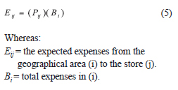
After statistically determining the criteria, the model can be used to forecast the consumer spending on a certain product provided by the store (j), which is located in a specific geographic area within the study area, according to the following formula:
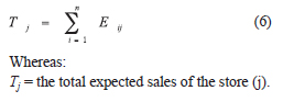
The total sales in each store in the geographical area can be determined by adding the expected expenses in each geographical area for all stores, according to the following equation;
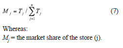
The market share of each store in the study area equals to the total expected sales of each store divided by the total sales of all stores, as follows:
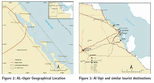
Steps of determining the study areaThe first and most important step after obtaining the relevant accurate data is to define the tourism impact area as it should be. This stage is very important due to the impact of geographic extension on determining the nature and volume of data that should be collected in addition to any conclusion to be reached based on the analysis of these data. The steps used to determine the impact area are illustrated as follows: 1. Locate Al-Uqair and similar tourism destinations, in addition to the road network and surrounding communities within the study area, which was identified in the third chapter of this study. 2. Determine the tourism impact area which depends on the distance traveled by tourists to reach the destination, assuming that the distance ranges from (100 km) to (400 km). This type of tourism involves a large group of local and regional tourists, and classified as medium-range tourism (Kafi, 2008). 3. Define the borders of the initial impact area, which usually reflects the natural or human barriers that hinder tourism movement between specific areas, and impedes movement between the defined area such as international borders, seas, mountains, and road network. 4. Draw the borders of common areas of influence, and this is the initial approximation to the impact area. 5. Divide the initial impact areas to smaller geographical units through which tourism statistics data could be collected. To determine these smaller geographical units, the previously identified sub-regions are usually used by some entities such as the Department of Census which divides the regions into different levels of spatial details. 6. Obtain the available tourism statistics for each sub-region which include the number of one-day trips, excursions, leisure trips, marine trips, the spending on marine activities, and the required location data (coordinates of latitude and longitude) for mapping each sub-region. 7. Modify the impact area if necessary to reflect the sub-region boundaries. 8. Collect data reflecting the relevant competitiveness of each tourism destination within the impact area such as the area, number of resorts and other tourism attractions. 9. Determine the distances or travel time between the sub-regions and all tourism destinations within the impact area. Application on study caseGeographical location Al-Uqair is located on the Gulf Sea coast in the Eastern Province of the Kingdom. It is located within Al-Ahsa administrative area. Al-Uqair coast extends between the latitudes (24’ 25 ) and (44’ 25 ) to the north, and between longitudes (50’ 08º) and (24’ 50 ) to the east. It is 50 km long, and 10 km wide inward. See Figure (2).
The tourism significance of Al-Uqair beach lies in its expected role. Its natural components imposed the merging of this beach on the national tourism map in Saudi Arabia, in addition to the likelihood of attracting a large number of visitors and tourists in the future. This means that the development of Al-Uqair beach will relieve pressure on other beaches in the eastern region. Moreover, new investment opportunities, and other economic and social returns are expected (SCTA, 1425).
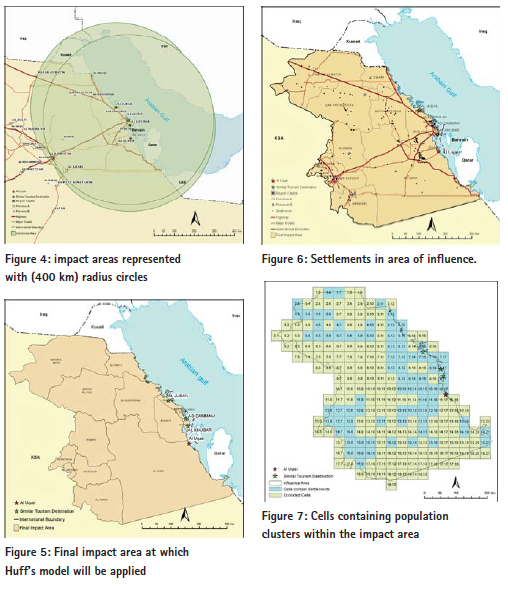
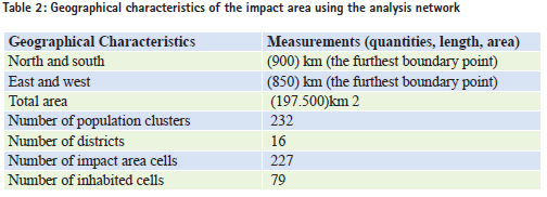
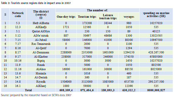
In step (1), Al-Uqair location and other similar tourism destination were determined. There are some tourism centers in the eastern coast which were developed partially or completely, such as Al-Jubail Industrial Corniche, Al-Dammam Corniche, Al-Khober Corniche, Al-Azizia and Half Moon. Similar destinations are located in Al-Dammam, Al-Khober, and Al- Jubail, and can be considered competitive centers for Al-Uqair beach, Figure (3). Step (2) describes the three competing tourist destinations for Al-Uqair and their areas of impact. They are forecast by circles of (400 km) radius, as shown in Figure (4). Step (3) shows the final boundaries of the tourism impact area, as shown in figure (5), after being adjusted in accordance to the provincial boundaries. The aim is to facilitate access to the available statistical tourism data at the district level (polygon). Figure (6) shows the population clusters with over (2,500) people, which is linked to the road network. Their total number reached (232) points, administratively distributed on (16) districts within the borders of the impact area. It is clear that the pattern of the spatial distribution of population points ranges between the clustered and random pattern. Using cellular representationBy covering the impact area with cellular network helps to calculate the area with square kilometers per unit (cell) in the map. It also helps in measuring the distances required by the Huff model. The selected cell size in this study is (50 X 50) square kilometers, to be compatible with the geographic data representation level at the regional level, and takes into account the spatial distribution pattern of communities. Thus, each cell could contain the largest number of communities, considering the center of each cell to be the distance measuring point to various tourist destinations. 148 cells were excluded because they do not contain any community. So, the total number of cells that contain population clusters is 79 cells within the impact area, as shown in Figure (7). Concluding the Characteristics of the Tourism Impact AreaTable (2) summarizes the geographical characteristics of the impact area by using the cellular model. It is clear that the tourism market options are limited to three destinations competing on an area of 197.500 square kilometers, and 232 population clusters in (16) districts. Tourist properties may vary among tourism trips exporting provinces depending on the differences in cultural and socio-economic backgrounds, besides the provided recreational activities. Table (3) shows the data of trip source, the number of one-day tourists, the purpose of trips whether for holidays and recreation or voyages; and the tourist spending on marine activities geographically distributed on (16) provinces. It is notable that the pattern of data distribution in the source regions, within the impact area, has no effect on the calibration of the model. However, its role is limited to determining the characteristics of potential tourists.
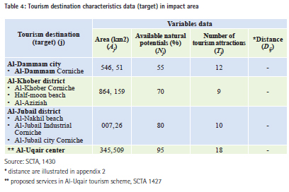
Analysis and discussionThere is an important factor to determine the impact of any tourist center on the communities which is the availability of other similar entertainment centers. Usually the proximity of tourist destinations to population clusters impacts the beach visitors. Although all destinations seem equal, the central tourism destinations are easily accessed and are likely to attract more tourists compared with other destinations. The attractiveness of tourist destinations, in most cases, is determined according to the variables that can be controlled by development officials as illustrated in the previous chapter. However, the variables used in this case study are limited to – spatial proximity, the area of the destination, and the availability of natural potentials and surrounding tourism attractions. Table No. (4) clarifies the characteristics of three tourism destinations: Al- Dammam; Al-Khober and AL-Jubail. It is clear that Al-Khober covers the largest area, followed by AL-Dammam and then Al- Jubail. Al- Jubail is featured by the available natural components such as pure sea water, and sandy beaches. Other tourism attractions are equally available in all destinations. Al-Uqair data was limited through the tourism development scheme and the results of the model’s coefficients calibration will be applied later.
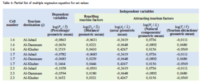
Calibration of the Huff model coefficients to forecast the tourism demandAfter collecting the tourism demand potentials’ data, which is necessary to calibrate the coefficients of the Huff model, equation (4.10) can be applied which represents the linear version of the Huff model. Table No. (5) shows a sample of regression equation data, including 9 data cells. The third column shows the dependent variable, representing the tourism demand potentials’ data divided by its geometric mean. Columns 4-7 show the independent variables arranged successively as follows – distance, area, natural components, tourism attractions, divided by its geometric mean.
Table (6) shows four attempts to calibrate the model. It used another type similar to the multiple regression called the Stepwise Regression, which determines the importance of each independent variable in explaining the change that occurs in the dependent variable. The ratio of change is ordered based on the importance of each independent variable. The order starts from the highest percentage, or the most important variable, and ends with the lowest ratio or the least important variable in explaining the change that occurs in the dependent variable. The fourth statistical model explains the four independent variables (*) (96%) of the variance in the value of the dependent variable (**). The variable of proximity is the most important variable to forecast the attractiveness of the tourism destination selected, representing (69%). On the other hand, the remaining tourism attractions variables have also high statistical significant.
Coefficients estimationTable No. (7) shows the forecasted coefficients, used as adjusted weights for the tourism attractiveness variables coefficients entered in the Huff model to forecast tourism. The distance coefficient weight ( ) represents the value (-2 ‚86), and minus sign indicates diminishing the impact with increasing distance. While the the natural components ( ) represents the value (12‚1), and the tourism attractions ( ) represents the value (66‚1). The positive variables coefficients indicate an increase along with the increasing variable. After obtaining the results of the coefficients calibration of variables, they will serve as modified weights. It is clear from Table (6) and Table (7) that the fourth model is statistically adequate for prediction, based on the value of the increasing determination coefficient (R2 = 0.9665) This indicates that the tourism demand in tourism destinations depends heavily on the variables given by the model. This is one of the methods used to evaluate the model. In addition, the significance level of the correlation coefficient reached zero (0.00), which is less than the significance level of hypothesis (0.05). Therefore, the regression line matches the data, which is within the limits used by geographers and others when accepting or rejecting the hypothesis that is usually in the limits of (0.50). So, after verifying the efficiency of statistical calibration, coefficients values will be used (adjusted weights) to forecast the tourism demand potential.
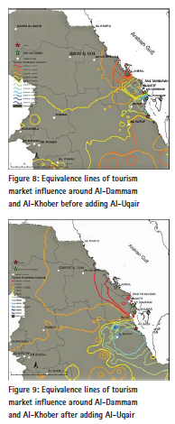
The resultsDetermining Al-Uqair tourism market share Visual evaluation of the tourism impact area and tourism market share for tourism coastal destinations can be obtained by comparing the equivalence lines of tourism market influence in the destinations before and after adding Al-Uqair destination. Figure (8) shows tourism market influence lines to of Al-Dammam and Al-Khober together before adding Al-Uqair. There is a clear overlap in their influence lines, while Al-Jubail was not added because of its relative faraway distance from Al-Uqair.
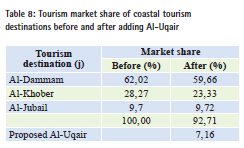
Figure (9) shows the influence lines of the tourism market in the existing tourist destinations after adding Al-Uqair. The differences in the distribution pattern of the lines after adding Al-Uqair is clear. It may be difficult to assess the impact visually, due to the large and overlapping equivalent lines. Al-Uqair share of the current tourism market can be determined. Table (8) indicates the quantitative estimation of the market share in the three existing tourist destinations within the tourism impact area. It is expected to distribute Al-Uqair market share between four tourism destinations after adding Al-Uqair instead of three tourism destinations. This can be identified through the application of the values of tourism demand potentials on the expenditure data for all source regions. The second column in the table clarifies the tourism market share before adding Al-Uqair. It is observed that the highest share of the current market belongs to Al-Dammam, followed by Al-Khober and then Al-Jubail. While the third column shows the potential tourism market after adding Al-Uqair. It was obtained using equation number (4.5). We note that all destinations have lost a part of tourists’ frequent visits. The forecasted loss of tourist destinations is approximately (-7.16%) from current tourists spending which will go to the new destination (Al-Uqair).
ConclusionThis study showed that the full potential of the Huff model has not been recognized yet. Adding to the Huff model in the business analyst program in (ArcGIS), the package is a positive step in this direction. There are many applications for this model not only in the field of tourism demand, but in other tourism aspects. For example, analyzing the tourism impact areas, assessing tourism market penetration, estimating the tourism development impact, assessing the tourism environmental impacts, predicting tourist preferences, and finally describing the tourists’ distribution patterns geographically. The study recommended the possibility of circulating the application of the model to tourist destinations similar to Al-Uqair in various regions of the Kingdom. The results of the Huff model coefficients calibration are applicable to several tourist destinations without making any changes. Running the proposed model’s progress scheme is fast and practical and saves a lot of effort and money, only in case of compliance with the terms and objectives of the model in addition to the required level of details. ReferencesArabic references • Kafi, Mustafa Youssif (2008). Tourism Economics, Syria, Damascus. Dar Al-Redha Publications • Ghunaim, Othman Mohemmed (2003). Tourism Planning for Comprehensive and Integrated Spatial Planning. Jordan, Dar Al-Safa Publications • Saudi Commission for Tourism and Antiquities (1425). Tourism Development Strategy for The Eastern Province. Kingdom of Saudi Arabia. Riyadh. Not published • Saudi Commission for Tourism and Antiquities (2007). Tourism Statistics. First edition. Kingdom of Saudi Arabia. Riyadh. Tourism Information and research Center Foreign references • Hooper, H. (1997). Who’s Really Shopping My Store? Business Geographies, September, 34-36 (not available online) Hudman, L. E. (1980). Tourism: A shrinking world. Columbus: Grid Inc. • Huff, David.L. (1963). A Probabilistic Analysis of Consumer Spatial Behavior. William S. Decker. • Huff, David.L. (1964). Defining and Estimating a Trading Area. Journal of Marketing 28. pp. 34-38. • Huff, David. L. (2003). Parameter Estimation in the Huff Model. ArcUser, October-December, 34-36 • Huff, David. L. (2004). A Note on the Misuse of the Huff Model in GIS. Retrieved from www. mpsisys.com on January 16. • Huff, David. L. (2008). Calibrating the Huff Model Using ArcGIS Business Analyst. A ESRI 380 New York St. Redlands. CA 92373-8100. USA The paper was presented at the Eighth National GIS Symposium in Saudi Arabia during 15 – 17 April 2013. |

 –
–


 (4 votes, average: 3.25 out of 5)


Leave your response!