| Mapping | |
Point clouds and orthomosaics from photographs
This paper presents the first examples where point clouds and orthomosaics, generated from close range photographs, can help civil engineers on their studies |
 |
|
 |
|
 |
|
The three authors of this paper work at the Applied Geodetic Division of the National Laboratory for Civil Engineering (LNEC), in Lisbon, Portugal. LNEC is a state owned research and development institution founded in 1946. It works in the various domains of civil engineering (structures, hydraulic, geotechnics, environment, materials, among others), giving it a unique multidisciplinary perspective in this field. The main goals of the LNEC are to carry out innovative research and development and to contribute to the best practices in civil engineering.
The Applied Geodetic Division nowadays develops works in two domains: the geodetic surveying of large dams and other engineering structures for monitoring purposes, and the processing of digital images with applications in several domains, which includes the study of the evolution of pathologies in engineering works. Originally the processing of digital images made use mostly of the chromatic information included in the images (from satellite images to close range photographs). But recently it has evolved to extract information of the geometry of the objects by the generation of point clouds. This use of close range photographs (from distances of decimetres to a few meters), which started in the summer of 2014, looks very promising and we, the authors, are identifying possible areas where the use of point clouds and orthomosaics that can be of interest to our colleagues of LNEC, civil engineers mostly. This paper presents the first examples where point clouds and orthomosaics, generated from close range photographs, can help civil engineers on their studies. The photogrammetic products were all generated using the free opensource software Micmac (Multi- Image Correspondances, Méthodes Automatiques de Corrélation) from IGN (Institut National de l’Information Géographique et Forestière, France).
First study case. The “introduction to point clouds”
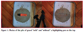
Although many colleagues, civil engineers, know the concept of “point clouds” we felt that we should generate a small point cloud example, light to manipulate: we called it “introduction to point clouds”. We were not innovative with the object chosen: we reproduced the example “Gravillon” of Micmac (Pierrot-Deseilligny, 2014): it creates a point cloud from a small pile of sand. Our example has a difference to “Gravillon” example: we embedded a highlighting pen on the top of the pile that was removed to study how differences between point clouds and orthomosaics can be detected. We created the first point cloud, the “with” point cloud, from a set of nine photos. Then, after, the pen was carefully removed and we took a second group of nine photos to generate the second point cloud: the “without” point cloud. In Figure 1 one can see two of the photos taken. Using these two clouds we could not only present the concept of point cloud but also we demonstrated that it was possible to detect differences between the clouds using (open-source) software.
The steps of the work, including the cloud comparison were:
Preparation of the sample
Inside a small tray we placed a paper with some straight lines drawn. As we know their length we established our “Ground Control Points” (GCP) in the intersection of the lines. On it we put some small dimension size gravel borrowed by the Geotechnique Department of LNEC. On the top we embedded a pen.
Taking the photos
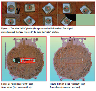
We used the digital camera Nikon D200, mounted on a tripod, with a lens with fixed focal length. The camera was set to manual mode (to keep focal length and aperture constants) and we took nine photos (Figure 2), JPG format, all about 1 meter of distance: one from the top, eight from the side. After this session we took other photos for calibration purposes.
Building the “with” point cloud.
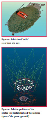
To build the cloud we followed the steps used in Micmac’s “Gravillon” example. These include (as presented by Pierrot- Deseilligny, 2011, and Samaan, 2013): i) common points search on pairs of photos; ii) computation of calibration parameters and geometric correction of the photos, determination of the position of the photos in a relative (not absolute) referential; iii) visualization of the positions and orientations of the camera in the relative referential establish previously (see Figure 6); iv) geo-reference of the data, to transform the relative orientation using the coordinates of three GCP well identified in the photos (points “A”, “B” and “C”, seen in Figure 1), either absolute coordinates in the 3D referential chosen and image coordinates in the photos; v) final computation of the external and internal orientations with data generated previously; vi) computation of the digital surface model, point cloud and ortomosaic (see Figures 3 and 5).
Building the point cloud “without”.
After taken the “with” photos we removed carefully the pen in order to keep the pile of gravel unchanged. We placed the tripod near the tray and took a new group of nine photos. We processed the information using the same software and following the same steps and we created the “without” cloud (see Figure 4).
To visualize the point clouds we used or Meshlab or CloudCompare (both opensource softwares). The background color (light cian) seen in Figures 3 to 5 was chosen to make the “holes” (= areas without points) more visible. These holes appear because is difficult for the software to find homologous points in surfaces too homogeneous (like the paper, the pen or its cap).
Comparing the clouds.
By comparing the clouds we expect that the depression, left by the pen when we took it out from the top of the pile, was visible (and could be somehow measured) by using software that compares the clouds. In this example is very obvious the change between the clouds. To perform the comparison we choose CloudCompare. As the clouds don’t cover exactly the same areas (for instance, the areas without points near GCP “A” and “B” have different shapes) we select, in both clouds and using Meshlab, circular areas in the XY plane with the same centre and radius. All the points whose location didn’t fulfil that condition were deleted. The new clouds were imported by CloudCompare and there we calculated the distance between the clouds. Before this computation CloudCompare presents some data, as seen in Figure 7. The point cloud chosen as reference was the cloud “without”. The largest distance between the clouds is 0. 0164 m (as seen in the form on the left side) and the majority of the points are at a distance lower than 0.002 m, according to the graph on the right and the colorized distances at the centre.
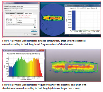
Selecting only the distances larger than 0.002 m a new image is obtained (Figure 8) that covers a smaller area since it is limited to the area near the pen (the distances in the majority of the circle were smaller than 0.002 m and for that reason not represented when the new image was created). On the left side of the Figure 8 is presented the frequency chart of the image.
Second study case. Natural rock joints
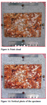
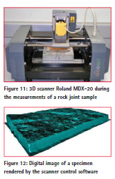
The Foundations and Underground Works Division (Concrete Dams Department) of LNEC carries out research studies that include the characterisation of the mechanical properties of rock masses and rocks. For this, in its Rock Mechanics laboratory, it conducts tests to obtain values to the parameters that characterize the deformability and the strength of rock specimens and joints. The case presented in this paper is one specimen of a rock joint (see in Figure 9 the point cloud seen from above, and in Figure 9 the vertical photo of the specimen) that had undergone a shear test to evaluate the influence of the normal and shear loads on the variation of surface roughness (in the case of rock joints, the roughness has a large influence on the shear strength).
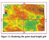
This specimen (a granite sample, 12×8 cm2) has been scanned with a three-dimensional scanner, as described by Resende and al. (2014), so we had 3D coordinates of its surface. The scan was made by the 3D needle-tip contact scanner Roland MDX-20 Figure 11) which allows the three-dimensional scan of solids (Figure 12). It was adopted a horizontal resolution of 0.5 mm. The scanning of the surface of the rock joint sample took eight hours.
We took nine photos of the specimen, following the methodology of the first case, with an innovation: the specimen was placed on a turning stand. This simple set decreased a lot the time that was spent on taking the photographs. With the nine photos it was created a point cloud and an orthomosaic. This one will allow studies never done before related with variations of the surface hue as a result of the shear test. As we didn’t have GCP, we defined a local reference frame by choosing a point to be the origin of the frame, and two lines to establish, one, the orientation of the frame and, the other, the scale.
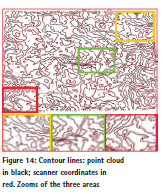
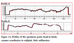
The surface of the specimen (the area with brown colors) was represented by 1647999 points with 3D coordinates. These can’t be directly compared with the 3D coordinates of the 38290 3D points surveyed by the scanner. So the first stage was to align the point cloud with the scanned data, done by the software Cloudcompare, which employs the algorithm Iterative Closest Point to minimize the difference between two clouds of points. The second was to generate a height grid. The third was to import this data by QGIS and explore the raster tools. In Figure 13 is presented the rendering of the point cloud height grid, in Figure 14 the contour lines (from the point cloud overlaid on those of the scanner) and, in Figure 15, two profiles lines, from the intersection of the vertical planes A and B (see their location in Figure 13) with the surface. Comparing the contour lines and the profiles small differences are noticeable.
Third study case. The model of a breakwater
Breakwaters in seaside areas are good examples of structures that can be monitored using the products derived from photographs taken by cameras mounted on unmanned aerial vehicles (UAV). The authors have presented in FIG Congress of 2014 an evaluation of the surface model of the breakwater of Ericeira (Henriques et al, 2014). The good results, especially if one takes into account the windy conditions during the flight, give us a good motivation to test the use of photogrammetry indoors, to help the studies of physical models of breakwaters belonging to the Harbours and Maritime Structures Division of the Department of Hydraulics and Environment.
Some of the studies of this division are on the structural behaviour of coastal protection structures, like breakwaters, under the action of waves. In tanks, different types of waves are reproduced, being that their height and period are set to reproduce the natural conditions of the sea that hits the structures. During the tests, that are several days or weeks long, there is a succession of periods of generation of waves followed by periods of pause, used to get information about the structure, namely the changes that affect its surface.
The aim of our study is to get answers to three questions: i) point clouds and orthomosaics can give accurate information on the behaviour of the models? ii) the generation of these products is time consuming? iii) how to get vertical pictures when the model is surrounded by water? At this moment we can answer to the first question with a “yes”. Concerning the other two we know for sure that is impossible, without the development of software, to perform a full automatic processing of photos because is necessary to get the coordinates of GCP on the photos, a phase that now demands the direct intervention of the user. Concerning vertical photos, we tested the use of an unmanned aerial vehicle (a small four rotors helicopter) that included a low quality camera. Despite its low quality, the photos were good enough to realize that helicopters is not the solution because the rotation of the propellers generated wind that produced agitation on the water surface and that affected the vision of blocks located under water. The solution must be different.
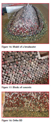
To get data to answer to the first question we chose a model of a rubble mound breakwater (2 m long, 1.3 m width and 0.3 m height, see Figures 16 and 17). The surface was covered with cubic blocks of concrete, painted in different colours, reused from other breakwaters models. The eight lower rows of blocks were covered with water. The photographs were shot vertically. The camera was at 3m high, fixed to a horizontal rod that was attached to a column. This column was supported on a structure with four wheels. The set moved on a platform that belongs to the model. The camera, the Nikon D200, was programmed to take photographs automatically every 10 sec during 10 minutes. In each position two photos were taken. After the first survey we moved some blocks manually and we made a second photo survey.
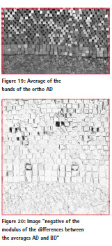
By applying Micmac we produced two orthomosaics (Figure 18), with a pixel size 0.32 mm in average, and two point clouds: a “before displacements”, BD, and an “after displacements”, AD. The orthos (raster images) were processed by QGIS. We used the “Raster Calculator” to: i) average the three RBG bands to generate two single band raster images (BD and AD, Figure 19); ii) to calculate the difference between these images; iii) to calculate the “square root of the square of the difference” (mathematical operation used when the function “modulus” is not available), operations that highlight the differences (see in Figure 20 the negative of the image created). The areas with differences are presented with darker grey. A more detailed description of the work can be found in Henriques et al., 2016.
Fourth study case. Visual inspection of wall of a dam
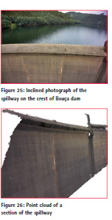
Some signals of deterioration and cracking of dams can only be identified by visual inspections. For this reason, these are irreplaceable in the control of the safety of dams. Concerning the exterior walls, and sometimes also the crest, as there is no direct access to most of these areas, cameras and/ or binoculars are used to perform the inspection work, which is usually done from the banks of the river. In our test we used photos taken by a digital camera carried by an unmanned aerial vehicle (UAV) helicopter of a small area on the downstream face and of the spillway on the crest of Bouçã dam (Figures 24 and 25).
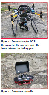
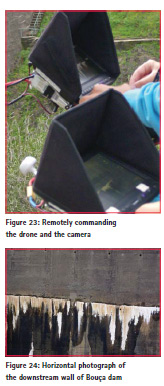
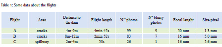
The photo survey was done by a digital camera Sony Nex-7, mounted under an eight-rotor mini helicopter (Figure 21, photo taken before the camera was mounted). The flight was remotely controlled by a pilot on the ground and there was a second technician who controlled the camera (its orientation and when to trigger). Each one had a remote control (Figures 22 and 23) that communicated with the drone. There were made three flights. Table 1 has a resume of the info of each flight. The first flight had to be interrupted due to a short shower, during which the heli was on land, protected from the rain.
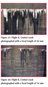
The dam has three major horizontal cracks, which are under surveillance since they were noticed. Two appear during the first filling, by 1956, the third in January of 2007. Due to the colour of the deposits of carbonates under the cracks, one can easily see their location. The change of the focal length allowed, without changing much the distance drone-wall, to have a group of images more global, better to produce an orthomosaic of the dam. On Figures 27 and 28 one can see the differences between the photographs taken with the focal length of 50 mm (flight A) and a focal length of 16 mm (flight B).
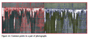
The first step of software Micmac is to detect common points in each pair of photos. In Figure 29 is presented the location of common points as detected by the software: one can see that it was difficult for the software to identify points in the white areas and in the wet areas.
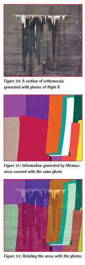
An orthomosaic is created by gathering selected areas of images, photos that were corrected from distortions of the camera and from the geometry of acquisition. In Figure 30 is presented a section of the orthomosaic generated by Micmac with the photos of flight B and, in Figure 31, information that helps to understand how the orthomosaic is built: an area with the same colour means that in that area of the orthomosaic it was used the same image (see Figure 32). In Figure 30 one can notice the frontiers between some areas; changing the value of a parameter of Micmac the final image could become more homogeneous. The main purpose of the flights was to collect data to support aided visual inspections. To evidence anomalies on the surface, digital image classification techniques were used to show the areas that shared the same characteristics. It was applied the technique known as “object-based image classification” to classify the anomalies represented in the orthomosaics and used the software eCognition from Trimble. The steps of classification were: i) segmentation: neighbour pixels were aggregated forming objects based on colour and shape (parameters defined by the user); ii) selection of variables and respective thresholds that provide an efficient identification of the features that are going to be classified; iii) automatic classification of the image.
The result of the classification is presented in Figure 33. One can see that three themes were chosen: i) white areas: deposits of calcium carbonate below the cracks where the water has leaked/is leaking; ii) red areas: areas where the calcium presents a redish colour; iii) wet concrete.
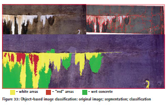
During the segmentation process, large and compact objects were formed respecting the radiometric borders visible in the image. Instead of performing the analysis of each individual pixel, the classification was applied over the objects. The objects representing areas with carbonates were identified through radiometric variables. The classification of the wet areas, besides the radiometry, also considered the proximity between the objects to be classified and those previously classified as carbonates. One can notice that some of the areas of the concrete that are darker were not classified as wet because its colour is not dark enough.
Conclusions
Point clouds and orthomosaics generated from photographs taken at short distances, less than 10 meters, can be helpful tools to experts like civil engineers that must made small scale studies. The examples presented were the first attempts and more studies on the accuracy must be performed. As a complement to the point clouds and orthomosaics, digital image processing techniques were verified to be great, providing useful information for Civil Engineering applications. In the presented examples, contributions to the identification of pathologies, detection of changes caused by natural elements and displacement evaluation were given.
References
Henriques,M.J. ; Braz,N. ; Roque,D. ; Lemos,R. ; Fortes,C.J.E.M. (2016). Controlling the damages of physical models of rubble-mound breakwaters by photogrammetric products – Orthomosaics and point clouds, Proceedings of the 3rd Joint International Symposium on Deformation Monitoring, Vienna. URL: http://www.fig.net/ resources/proceedings/2016/2016_03_ jisdm_pdf/reviewed/JISDM_2016_ submission_50.pdf
Pierrot-Deseilligny,M. ; Luca,L. ; Remondino,F.. 2011. Automated image-based procedures for accurate artifacts 3d modeling and orthoimage generation. XXIIIrd International CIPA Symposium. International Committee for Documentation of Cultural Heritage (CIPA).
https://www.conferencepartners.cz/cipa/ proceedings/pdfs/B-2/Remondino2.pdf
Pierrot-Deseilligny,M.. 2014. MicMac, Apero, Pastis and Other Beverages in a Nutshell! (Micmac manual). IGN. http:// logiciels.ign.fr/IMG/pdf/docmicmac.pdf
Resende,R.; Ramos,A.L.; Muralha,J.; Fortunato,E.; Lamas,L.. 2014. Characterisation and Numerical Modelling of the Geometry of Rock Joints. The 8th Asian Rock Mechanics Symposium.
Samaan, M. ; Héno,R. ; Pierrot- Deseilligny,M.. 2013. Closerange photogrammetric tools for small 3D archeological objects. XXIVrd International CIPA Symposium. International Committee for Documentation of Cultural Heritage (CIPA).
http://www.int-arch-photogrammremote- sens-spatial-inf-sci.net/ XL-5-W2/549/2013/isprsarchives- XL-5-W2-549-2013.pdf
Rosu,A.M.; Pierrot-Deseilligny,M.; Delorme,A.; Binet,R.; Klinger,Y.. 2014. Measurement of ground displacement from optical satellite image correlation using the free opensource software MicMac. ISPRS Journal of Photogrammetry and Remote Sensing.
http://dx.doi.org/10.1016/j. isprsjprs.2014.03.002


 (1 votes, average: 3.00 out of 5)


Leave your response!