| GNSS | |
The impact of the high ionospheric activity in the EGNOS performance
This article provides a summary of the different analyses performed by ESSP relative to the existing correlation between the EGNOS performance measured over the north region of the EGNOS service area, some ionospheric indicators and some solar events. |
 |
|
 |
|
 |
|
 |
|
 |
|
From the beginning of 2008, we have been facing a period of high solar activity linked to solar cycle #24. Taking into account a typical duration of eleven years, solar cycle 24 would have just reached halfway point. Figure 1 shows the evolution and prediction of different parameters used to measure the solar activity, number of sunspots (SSN) and the planetary geomagnetic indicator (Ap) that reflects the existence of a high geomagnetic activity in the ionosphere. From Figure 1, it can be deduced the smoothed monthly value of the number of sunspots reached a first maximum in February 2012. A second relative maximum, higher than the first one, was attained in August 2013. The increase in solar activity affects the geomagnetic behavior of the ionosphere.
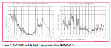
As it can be seen in Figure 1, the evolution of the Ap index, which provides an indication of the geomagnetic activity as measured by different magnetometers over Earth, does not present a link with the solar cycle as evident for other parameters. This is because a slight increase of the number is observed when a period of geomagnetic storms arrives.
The dependence of EGNOS performance with the variations observed in the ionospheric behavior is known (Billot et al., 2013), and has been relevant since the beginning of the solar activity increase linked to the current solar cycle. Such events affect not only EGNOS, but also other SBAS systems under geomagnetic storm conditions. This is considered as an intrinsic limitation in single frequency SBAS systems. The reason for this is that SBAS systems estimate ionospheric delays assuming a bi-dimensional behaviour of the ionosphere (no height). This is true in a nominal situation, but is not accurate in case of high geomagnetic activity or ionospheric storms, when the ionosphere behaves as a 3-dimensional body whose properties change with height.
In the past, some areas of Europe were more sensitive to the variations in the behaviour of the ionosphere. An improved level of stability has been currently achieved after the deployment of the EGNOS2.3.1i in August 2012. A new EGNOS release (2.3.2), deployed in October 2013, has increased the robustness of EGNOS against this kind of events, correcting some issues which were observed during autumn of 2012. However, even if this new release provides a high stability to ionospheric disturbances, some degradation can still be expected during periods with very high geomagnetic activity. Dual-frequency is expected to solve this issue, although scintillation may still be a concern in equatorial areas (Walter, 2012). Another important aspect, of the iono related SBAS performance degradations, is that they are highly location-dependent and the service status may vary for neighboring locations (FAA, 2013).
Several indicators can be used to measure the status of the ionosphere such as the K and A indexes or the SSN. The dependence of EGNOS performance with the indicators is known (Suard et al., 2013), and has been relevant since the increase of the solar activity in 2011. Other indicators, such as the disturbance storm time (Dst), are currently being investigated as an alternative mean to detect ionospheric events. The preliminary analyses of this indicator have demonstrated the presence of a high degree of reliability to detect ionosphericrelated events affecting SBAS systems.
Impact of ionospheric events in EGNOS performance
The evolution of the observed EGNOS performance since the beginning of this solar cycle has demonstrated that a close link exists between some of these parameters and the behavior of the ionospheric corrections provided by the system. This link is particularly clear in the case of performance degradations observed in the North of Europe, during periods with very high geomagnetic activity. In fact, this issue and its impact on the performance are well known since the beginning of the solar cycle for EGNOS and other SBAS systems.
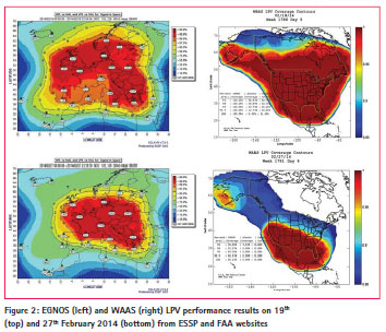
The month of February in the year 2014 represents a very clear case of a period with a high number of ionospheric events impacting the performance of EGNOS and other SBAS. As an example, Figure 2 presents the daily LPV performance achieved by EGNOS and WAAS during two particular degraded days, February 19th and 27th. Note that EGNOS LPV availability is measured as the percentage of time the Horizontal Protection Level (HPL) and VPL (Vertical Protection Level) are below the Horizontal Alarm Limit (HAL) and Vertical Alarm Limit (VAL). HAL is 40 m and VAL is 50 m for LPV. The International Civil Aviation Organization (ICAO) requirement specifies that availability must be over 99%.
As it can be observed, several regions in the North of Europe (EGNOS) and Canada (WAAS) were affected on February 19th. The case that occurred on February 27th is significant. During this day, the LPV coverage area obtained with both SBAS systems represents a small portion of the corresponding service areas (ECAC and CONUS respectively). Note that the observed impact during those days is relevant because ionospheric events cannot be notified to users (Pintor et al., 2013) in advance. Even if the possibility of predicting such a kind of phenomenon using space weather forecasts is still under investigation, the high impact for SBAS users show the clear need of understanding the mechanisms involved in this process.
The following section provides some information about the use of some public indicators to measure the ionospheric activity.
Ionospheric indicators to monitor EGNOS performance degradations
In this section, several geomagnetic indexes are presented and their correlation to EGNOS performance. Indexes used for monitoring the behavior of the ionosphere are:
• K/Kp index: The K index provides a representation of disturbances in the horizontal component of magnetic field, as observed on a magnetometer during a 3-hour interval. It is represented by an integer scale in the range 0-9: a value of 0 indicates absence of any disturbance. A value of 5 or above indicates geomagnetic storm. The planetary Kp index is obtained by averaging the K-indices from a set of geomagnetic stations.
• A/Ap index: The A index represents a daily average value of the geomagnetic activity measured at a specific station. It can be derived from the 3-hourly Kp indexes, following a transformation from a logarithmic to a linear scale. The Ap index is the averaged planetary A-index obtained using a set of stations over the whole planet.
• Dst index: Index of magnetic activity representing the intensity of the equatorial electrojet. It is obtained from a network of near-equatorial geomagnetic observatories.
• TEC maps: These are global maps of ionospheric Total Electron Content (TEC) obtained from observables from ground stations. This information is usually distributed using IONEX format files.
• Solar indexes: Some additional indexes are used to monitor the solar activity. Some of them are the Sun Spot Number (SSN), 10cm solar radio flux, proton flux, etc.
In particular, A/Ap and K/Kp provide a direct indication of the level of geomagnetic activity that can be used to analyze a potential correlation with the behavior of the Protection Levels obtained using the information provided by SBAS.
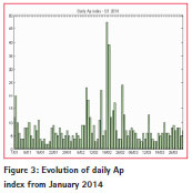
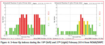
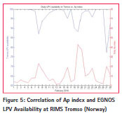
As already mentioned in the previous section, the month of February in 2014 presented some events with a high level of geomagnetic activity. This is visible in the Ap series evolution which shows several days with daily values of Ap above 20 (Figure 3). Note that an Ap index of 30 or greater indicates local geomagnetic storm conditions. In Figure 4, two peaks in the Kp index are clearly identified to present high value corresponding to the dates presented in Figure 2. These values confirm that during those days a high geomagnetic activity took place that explains the results observed in the LPV performance of both SBAS systems. The link with the behavior of EGNOS performance is clear if we fix the attention in the results measured at high latitudes. As an example, Figure 5 shows the dependence between the LPV availability measured in RIMS Tromso (located in Norway) and the daily Ap index, during February 2014.
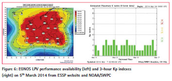
This case shows that a high correlation exists between the value observed in this Ap index and the results obtained in this station. Note, however, that the size of the impact is not always the same: some events are observed with a lower level of activity but a higher impact in terms of performance. Figure 6 presents an example, corresponding to the case on March 5, 2014, wherein the EGNOS performance degradation in the north of Europe is not linked to a high value of the Kp indicators.
However, the use of these indicators also presents some limitations:
– Temporal resolution: As the A/ Ap is a daily index, its use for the detection of geomagnetic events of short duration is not always the best option. This problem could partially be solved by using the 3-hourly K/ Kp indexes. But even in this case, the estimation of a geomagnetic storm is limited to an interval of 3 hours, that doesn’t seems adequate to identify any potential correlation with the instantaneous values of the Protection Levels obtained using EGNOS (calculated at 1Hz).
– Geographical applicability: The second limitation is linked to the fact that the Ap or Kp indexes correspond to global planetary values. This means that the values are obtained by averaging the values measured at different stations, which could be located at different longitudes and latitudes. If a geomagnetic storm occurs over the American continent, a decreased effect over Europe is likely; whereas the planetary indexes would be affected. As EGNOS is a local system limited to Europe, it would be necessary that this value be computed for a certain set of stations located over the ionospheric region supported by EGNOS. – Level of correlation: Finally, as commented above, even if the level of correlation is high when the results are observed, the link is not always so evident. Several cases are known in which the values of the Ap/Kp indexes present low values, even if the SBAS performance are disturbed. In the same way, several geomagnetic storms have a limited impact in the performance levels.
All these limitations show that the information provided by these indexes needs to be used carefully in order to understand the impact of the ionospheric behavior in the performance of SBAS.
The following sections present a detailed analysis of additional parameters and indicators which could be used in order to understand the close link existing between the ionospheric behavior and the performance observed by SBAS users.
Geomagnetic effects on EGNOS in the north of Europe
Horizontal error is bound by HPL and HPL is calculated with the EGNOS information broadcast according to MOPS 229D (RTCA, 2006). The EGNOS performance appeared to be degraded due to geomagnetic conditions during several periods in February 2014, with values of HPL well above the 40 m HAL. It is of great importance to emphasize that although availability was degraded in the North, EGNOS integrity was always guaranteed with every single epoch for the whole service area.
Approach to EGNOS degraded performance in the North in February 2014
As explained earlier, geomagnetic indicators show a relation between geomagnetic activity and SBAS performance (HPL). From (RTCA, 2006), it is known SBAS systems model its ionospheric corrections and integrity information from TEC estimated by its algorithms. TEC disturbances are known to also be correlated to geomagnetic storms (Mendillo, 2007) and local time (Biquiang et al., 2007). These storms at the same time can be traced to exchanges between the Earth’s magnetosphere and the interplanetary conditions originated by the Sun (Zhang et al., 2007). Space weather research is bent on understanding a series of phenomena that originated when the Sun liberates matter into the Solar System. These phenomena, whose description is out of the scope of this paper, include: coronal mass ejections (Webb, et al, 2012), solar flares (that can be B, C, M and X flares according to their brightness) (Hudson, 2011), coronal holes (Cranmer, 2002) and solar prominences and filaments (Van Ballegooijen et al., 1989). Moreover, the matter blown out from the Sun moves away from it in a continuous but varying flow and is called the solar wind. Finally, the magnetic field of the solar system, arising from the magnetic activity of the Sun is called the interplanetary magnetic field (IMF).
In order to analyze the geomagnetic conditions in February, the method of analysis focuses on the negative variations of interplanetary magnetic field z component (Bz), and the solar wind speed sudden increases. More information on this method can be found on (Zhang et al., 2007). We have tried to identify the correlation with EGNOS HPL in Tromso, ROTI in the North of Norway and Earth’s magnetic field in Tromso. All these five variables were retrieved from the following data sources:
– EGNOS data source: Apart from the fault-free monitoring method, EGNOS user performance (Integrity, Accuracy, Availability and Continuity) is monitored daily by the ESSP EGNOS Mission Performance Team (Roldan et al., 2014) for a list of EGNOS RIMS (Ranging and Integrity Monitoring Station) that provide observation data with a frequency of 1Hz. Several RIMS within the service area are located in Northern Europe (Egilsstadir, Kirkenes, Gävle, Lappeenranta, Reykjavik, Trondheim and Tromso) whose data is available at EDAS FTP (EC, 2013). For this study, RINEX data from Tromso (69.65°N) in Norway have been selected in order to compare with other available ground data sources. For this analysis, it has computed the value of the HPL obtained at this station using the information provided by EGNOS. Horizontal error is bound by HPL and HPL is calculated according to MOPS DO-229D.
– Rate of TEC index at ground (ROTI) data source: Norwegian Mapping Authority (NMA) operates a network of permanent GNSS stations. Based on the data collected from these stations (Jacobsen et al. 2012), the NMA Real-Time Ionosphere Monitor (RTIM) estimates the state of the ionosphere providing, among others, online ROTI and TEC graphs in Norway. ROTI data for this study has been provided on demand by NMA.
– Earth’s Magnetic field data source: Tromso Geophysical Observatory (TGO) (Johnsen, 2013) operates the Tromso magnetometer and several others along the Norwegian coast and on Svalbard. TGO provides graphical, historic and real-time data on their website. On demand, they can provide numerical data as they have done for the present study.
– IMF and solar wind speed data source: Advanced Composition Explorer (ACE) spacecraft (Stone, 1998) observes particles of solar, interplanetary, interstellar, and galactic origins, spanning the energy range from solar wind ions to galactic cosmic ray nuclei. From a vantage point of approximately 1/100 of the distance from the Earth to the Sun, ACE performs measurements over a wide range of energy and nuclear mass under solar wind flow conditions, and during both large and small particle events including solar flares. ACE provides near-real-time solar wind information over short time periods. ACE data can provide an advance warning (about one hour) of geomagnetic storms. For the present study, solar wind speed in GSM coordinates and interplanetary magnetic field data have been retrieved from NOAA FTP.
Detailed analysis of EGNOS performance
In February 2014, the EGNOS performance presented several periods that can be considered highly degraded. For detailed analysis, three time periods have been selected: 7th to 13th, 18th to 20th, and 27th to 28th. When analyzing the events, it has been decided to sort them according to the HPL degradation they produced becoming Event #2, Event #3 and Event #1, respectively.
Event #1: February 27th to 28th
The first period of analysis starts at 1700 UTC on February 27, when EGNOS performance degraded in the North of Europe. At that time, geomagnetic indexes did not react immediately since Kp index was 4 at the next calculation slot (1800UTC) and only jumped to 6 (major storm) at 2100 UTC. Dst was only slightly negative at the next calculation epoch (-8nT at 1800UTC) and then dropped to -99 nT at 2300 UTC.
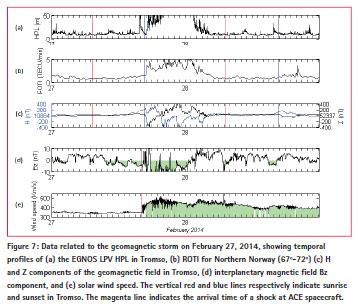
Figure 7a shows how EGNOS LPV HPL in Tromso rose on the 27th from 1715 UTC to 28th 0200 UTC, exceeding the HAL. Figures 7b and 7c show time profiles of ROTI in Northern Norway and the variation of the horizontal (H) and vertical (Z) Earth’s magnetic field measured in Tromso. Both HPL and ROTI showed clear high (disturbed) values from approximately the same time (1700 UTC). Earth’s magnetic field variations seem to start even before (1500 UTC).
On taking a look at the interplanetary information measured by ACE, the solar wind speed is illustrated in Figure 7d and the IMF north-south (Bz) component in Figure 7e. In Figure 7d and Figure 7e, light green shading means that Bz is negative and solar wind speed is above 380 km/s respectively. When it comes to the data, in Figure 7d, a sudden jump in the solar wind speed (from 350 km/s to a maximum 520 km/s at 1930 UTC) is detected by ACE at 1609 UTC marked by a vertical magenta line. Moreover, IMF north-south (Bz), which was already mainly negative during the previous six hours, started flickering at 1600 UTC and finally dropped to almost -20nT at 1800 UTC. It remained negative until 0200 UTC.
From the analysis above, it seems clear that the disturbed conditions started one hour after the arrival of the shock detected by ACE at 1609 UTC, which by its locations must receive the shock one hour before Earth. According to (NOAA, 2014a), this shock on February 27th is a consequence of the coronal mass ejection associated to a X4.9 flare erupted from the Sun at 0049 UTC on February 25th.
Event #2: February 7 th to 13 th
A second period of interest was identified from February 7th to 13th where a series of degradations affected EGNOS user’s during night-time from 7th to 12th. The case of February 13, considered a day with EGNOS nominal performance, is also included in the analysis as a nominal reference.
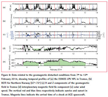
Figure 8a shows different levels of EGNOS performance degradations during the nights from 7th to 12th. Periods of higher and more degraded HPL are presented on the 9th and 10th. These periods become shorter on the 12th. Figure 8b shows a similar trend for ROTI in Northern Norway and in Figure 8c, it can be seen as Earth’s magnetic field is also affected in a similar manner. This confirms the Figure 7 analysis. For this week, Kp index reached 5 (minor storm) at 2100 UTC on the 9th and then stayed between 2 to 4 during the rest of the period. In (NOAA, 2014b), it identified the arrival of two shocks at ACE, one at 1616 UTC on the 7th (due to the arrival of the coronal mass ejection associated to M3.8 flare) and the second one at 1900 UTC on the 10th, due to the arrival of coronal hole high speed stream (Kavanagh et al., 2007) according to (NOAA, 2014c). Both shocks are marked by a vertical magenta line. From Figure 8d, other two situations where solar wind speed jumps took place at 1100 UTC on the 9th and 1800 UTC on the 11th. At the same time, the IMF Bz turns negative (Figure 8e). In Figure 8d and 8e during the night of the 8th to the 9th, the effects over HPL, ROTI and Earth’s magnetic field of a relatively not-so-high solar wind (400Km/s) and a persistent negative Bz (lasting 17h) can be seen.
It is also interesting that the effects of a higher solar wind speed (maximum of 570 km/s) on the night of the 9th to 10th did not produce such high HPL or ROTI values. The different effects over HPL and ROTI seem to be related to the strength of the combination of solar wind speed, and either the flickering Bz (lower effects) or full negative Bz (greater effects) peaking at midnight.
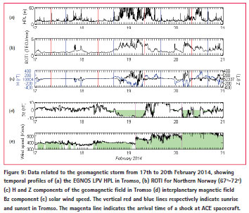
Event #3: February 18th to 20th
Finally, on February 18th, Figure 9d shows an increasing negative component of the IMF Bz since 1300 UTC. Bz stabilizes at -9nT at 2100 UTC. For the same period, the solar wind speed is above 400 km/s.
The effect of this combination is clear in HPL (Figure 9a), ROTI (Figure 9b) and Earth’s magnetic field (Figure 9c). According to the previous cases, this should have produced an increase HPL and ROTI during the nighttime at Tromso, but when daylight arrived, HPL should have come down to a much lower value. However, at 0309 UTC, a shock, probably because of a coronal mass ejection on the 16th (NOAA, 2014d), arrived at ACE making the solar wind speed rise to 500 km/s with a maximum of 550 km/s. The solar wind speed stays over 400 km/s until the end of the plotted period. The IMF Bz, already quite negative, plummeted and reached a minimum of -15nT. Bz stayed negative until 0800 UTC. Bz finally started flickering until 1300 UTC. This storm made Kp index reach 6 (major storm) for several intervals on the 19th, and Dst decreased to a minimum of -112nT at 1200 UTC that day.
What makes the effects of this storm different from previous cases is that the disturbed HPL, ROTI and Earth’s magnetic field continued during daylight on the 19th. So it seems that the combination of more disturbed values of solar wind speed and negative Bz can extend the effects over HPL and ROTI to daylight. A similar situation happened on the 20th, when ACE spacecraft detected a sudden increase of solar wind speed from 500 km/s to 650 km/s with a peak of 750 km/s, probably due to a filament eruption on the 18th (NOAA, 2014d), at 0251 UTC. IMF Bz again plummeted and the effects could be appreciated during daylight in Tromso.
Conclusion
A summary of the different analyses performed by ESSP relative to the existing correlation between EGNOS performance measured over different regions of the EGNOS service area and some of those ionospheric indexes (Kp, Ap, etc…) is presented in the article. Even if the use of those basic indicators provides good results in general, the correlation between those parameters and EGNOS LPV performance is not always direct. The existence of some limitations justifies the search of additional sources of data that could provide a better match with the observed results.
With this objective in mind, ESSP is advancing towards a deeper understanding of the effects of ionosphere at user performance level. In the present study, limited to some events in February 2014, ESSP Mission performance team has identified the existing link between EGNOS LPV performance outliers and variations in the ROTI, Earth’s magnetic field, solar wind speed and IMF Bz component. As a result of this analysis, the existence of a joint effect of the high solar wind speed plus a negative (or even disturbed) IMF Bz over degraded EGNOS LPV HPL has been identified. This same joint effect is used in literature to confirm the effects of geomagnetic storms. Also, it is shown, that ROTI, HPL and Earth’s magnetic field are mainly disturbed simultaneously.
More analysis must be done to confirm early conclusions, but the variations in these parameters seem to be correlated to EGNOS LPV performance in a promising way. Shock detection at the ACE spacecraft, where typically disturbed conditions arrive at about 1 hour before the Earth, and other sources of information (i.e. SOHO/LASCO) must be assessed as an early warning of performance degradation in the North of Europe
Acknowledgments
The authors wish to thank the providers of data used in the present study. We thank Dr. Knut Stanley Jacobsen from the NMA for the ROTI data. We also thank Dr. Magnar G. Johnsen from Tromso Geophysical Observatory for the Tromso magnetic field data. ACE IMF data, solar wind speed data, Kp index and Weeky reports were obtained from the NOAA Space weather prediction center. Dst index was retrieved from the World Data Center for Geomagnetism (Kyoto).
References
Billot A. and Schlüter S. (2013). Impact of strong ionospheric conditions over EGNOS and mitigation actions, BSS2013 proceedings, Bath, UK.
Biquiang Z., Weixing W., Libo L, and Tian Mao (2007). Morphology in the total electron content under geomagnetic disturbed conditions: results from global ionosphere maps, Ann. Geophys., 25, 1555–1568, 2007.
Cranmer S. (2002). Coronal holes and the solar wind, Yohkoh 10th Anniversary Meeting proceedings, Kailua-Kona, USA.
Federal Aviation Administration (2013). WAAS Technical Report DR #115 Effect on WAAS from Iono Activity on June 1, 2013. WAAS Technical Report William J. Hughes Technical Center Pomona, New Jersey. USA.
Hudson H. (2011). Global Properties of Solar Flares, Space Science Reviews, vol. 158, no. 1, pp. 5-41.
Jacobsen, K. (2012). Observed effects of a geomagnetic storm on an RTK positioning network at high latitudes, J. Space Weather Space Clim., 2012, 2, A13.
Johnsen, M. (2013). Real-time determination and monitoring of the auroral electrojet boundaries, J. Space Weather Space Clim., 2013, 3, A28.
Kavanagh A. and Denton M. (2007). Highspeed solarwind streams and geospace interactions, Astronomy & Geophysics.
Mendillo, M. (2006). Storms in the ionosphere: patterns and processes for total electron content, Rev. Geophys., 44, RG4001, doi:10.1029/2005RG000193.
NOAA (2014a). Preliminary Report and Forecast of Solar Geophysical Data SWPC PRF 2009 03 March 2014. NOAA (2014b). Preliminary Report and Forecast of Solar Geophysical Data SWPC PRF 2006 10 February 2014.
NOAA (2014c). Preliminary Report and Forecast of Solar Geophysical Data SWPC PRF 2007 17 February 2014.
NOAA (2014d). Preliminary Report and Forecast of Solar Geophysical Data SWPC PRF 2008 24 February 2014.
Pintor P., Rodriguez A., Jimenez F., Garcia A. and Gavín A. (2013). GNSS Performance Based Navigation Procedures Validation, ENC 2013 proceedings, Vienna, Austria.
Roldan R., Pintor P., Gomez J., De la Casa, C., Fidalgo, R. (2014). The EGNOS Performance monitoring activities performed by the ESSP, ENC 2014 proceedings, Rotterdam, The Netherlands.
EC-European Commision (2013). EDAS Service Definition Document.
RTCA-Radio Technical Commission for Aeronautics (2006). DO229D Minimum Operational Performance Standards for Global Positioning System/Wide Area Augmentation System Airborne Equipment’, RTCA 229D.
Stone, E., Frandsen, A., Mewaldt, R, Christian, E., Margolies, D., Ormes, J and Snow, F. (1998). The Advanced Composition Explorer. Space Science Reviews, v. 86, Issue 1/4, p. 1-22.
Suard N., Carvalho F., Rifa E., Mabilleau M., Robert E. and Yaya P. (2013). Solar cycle 24 activities first Impacts on SBAS, ENC 2013 proceedings, Vienna, Austria.
Van Ballegooijen A. and Martens P. (1989). Formation and eruption of solar prominences, Astrophysical Journal, Part 1, vol. 343.
Walter T. (2012). The Impact of the Ionosphere on GNSS Augmentation, ION GNSS 2012 proceedings, Nashville, USA.
Webb D. and Howard T. (2012). Coronal Mass Ejections: Observations, Living Rev. Solar Phys.
Zhang J., Richardson I., Webb D., Gopalswamy N., Huttunen E., Kasper J., Nitta N., Poomvises W., Thompson B., Wu C., Zhukov A. and Yashiro S. (2007). Solar and interplanetary sources of major geomagnetic storms (Dst <100 nT) during 1996–2005, Journal of Geophysical research, Vol 112.


 (7 votes, average: 3.29 out of 5)


Leave your response!