| Applications | |
Mapping the urban atmospheric carbon stock
We present this study in two parts. In this part, the materials and methods are discussed. The results of the study will be published in May 2022 issue of Coordinates |
|
|
|
|
|
Abstract
Currently, the worsening impacts of urbanizations have been impelled to the importance of monitoring and management of existing urban trees, securing sustainable use of the available green spaces. Urban tree species identification and evaluation of their roles in atmospheric Carbon Stock (CS) are still among the prime concerns for city planners regarding initiating a convenient and easily adaptive urban green planning and management system. A detailed methodology on the urban tree carbon stock calibration and mapping was conducted in the urban area of Brussels, Belgium. A comparative analysis of the mapping outcomes was assessed to define the convenience and efficiency of two different remote sensing data sources, Light Detection and Ranging (LiDAR) and WorldView-3 (WV-3), in a unique urban area.
The mapping results were validated against field estimated carbon stocks. At the initial stage, dominant tree species were identified and classified using the high-resolution WorldView3 image, leading to the final carbon stock mapping based on the dominant species. An objectbased image analysis approach was employed to attain an overall accuracy (OA) of 71% during the classification of the dominant species. The field estimations of carbon stock for each plot were done utilizing an allometric model based on the field tree dendrometric data. Later based on the correlation among the field data and the variables (i.e., Normalized Difference Vegetation Index, NDVI and Crown Height Model, CHM) extracted from the available remote sensing data, the carbon stock mapping and validation had been done in a GIS environment. The calibrated NDVI and CHM had been used to compute possible carbon stock in either case of the WV-3 image and LiDAR data, respectively. A comparative discussion has been introduced to bring out the issues, especially for the developing countries, where WV-3 data could be a better solution over the hardly available LiDAR data. This study could assist city planners in understanding and deciding the applicability of remote sensing data sources based on their availability and the level of expediency, ensuring a sustainable urban green management system.
1. Introduction
To date, rapid urbanization intensely poses the need for greener landscapes in many urban areas worldwide. Green spaces allow maximizing urban resilience and livability and to positively respond to climate change effects. While cities are striving for more green space, more than half of the earth’s population is already living in cities, and by 2050, 66% will be city dwellers [1]. Overexploitation of environmental resources for the huge population is indeed increasing the vulnerability of the urban dwellers to natural hazards.
To keep pace with rapid urbanization, efficient urban green planning could be nothing but a time being and an expeditious solution. Conservation and expansion of existing urban vegetation based on their structural and functional roles in an urban atmosphere are some of the most effective factors of green urban planning. Thus, various approaches based on advanced technologies have been implemented to assess the contributions of urban trees, especially evaluation of their roles in atmospheric Carbon Stock (CS) is being increasingly acknowledged [2,3]. Trees in city streets and parks are now being recognized as a key tool against impacts caused by the increased rate of atmospheric carbon dioxide (CO2) concentrations [4–7], since they sequester atmospheric carbon during the whole growth process and at the same time delay the adverse effects of climate change contributing to the accumulation of carbon in the soil [8– 10]. Studies found that the total yearly reduction in carbon emission can be up to 18 kg/tree in urban areas [11–13], which clearly brings out the importance of planting trees along with having an efficient tree management policy, especially in a complex city environment. Trees directly impact atmospheric CO2 fixation through photosynthesis, but in urban areas, the process is quite fitful due to tree health issues. As it is well known that the well-grown trees store far more carbon than the poorly grown ones, in urban areas, it is a huge challenge to maintain and preserve mature trees and well-managed urban forests that also include tree plantations and replacements. Therefore an efficient and timewise monitoring approach is essential to introduce an adequate urban tree management system [14,15]. In addition an effective monitoring system could be ensured utilizing an accurate and convenient species-based CS mapping approach. Most of the CS calibration and predictive models are based on the estimation of Above Ground Biomass (AGB) production [13,16–20], which is considered to be primarily responsible for the atmospheric CS [10,21–23]. In this study, the AGB was estimated based on the tree allometric information (i.e., Height (H), Diameter at Breast Height (DBH)) collected during the field surveys.
Currently, remote sensing-based mapping has been availed as an influential approach in monitoring functional and structural urban tree features to policymakers [24–31]. In fact, spatially extracted information on tree species and habitats over large areas are significant in understanding species’ roles, such as in providing ecosystem functions and services [32–35]. Over the last few decades, remote sensingbased classification of tree species has been widely utilized either in the case of mapping specific species-based ecosystem services (ES) outcomes (i.e., [36]), or growth and yield models and, etc. (e.g., [33,37,38]). Remote sensing approaches, especially hyperspectral imagery, have significantly upgraded the tree classification outcomes either in single trees or mixed populations [33,39– 43]. The utilization of very high spatial resolution multispectral satellite imagery (e.g., 1-m IKONOS, 0.6-m QuickBird) and aerial photos/digital imagery has been rapidly increased, especially in spatial mapping [44–47]. As a matter of fact, recently, with the advancements of remote sensing technologies, a diversified type of very high resolution remotely sensed images (such as WorldView-3, WV-3) are commercially available, certainly introducing a wave of opportunities for the accurate mapping of urban trees at a significant level [31,33,48–52]. Moreover, in the case of this study, a high-resolution WV-3 image has been successfully utilized to classify the dominant tree species in Brussels, which has been found useful for further CS mapping as it was earlier in the case of Sassuolo [36].
Additionally, there are also many convincing applications of Light Detection and Ranging (LiDAR) based calibration of the tree CS utilizing the individual tree metrics (i.e., [53–61]). On the other hand, much less evidence is available in the CS calibration of the urban trees utilizing only the multispectral satellite data [11]. In the case of urban areas, tree species mapping is still a considerable challenge due to having spatially heterogeneous land cover types from isolated trees to the dense forest, high tree species diversity along with heavily and regularly managed trees, as well as the interruptions by buildings and their shadows [7,62– 66]. Considering these facts, Geospatial Object-Based Image Analysis (GEOBIA) has been utilized in this study to classify the dominant tree species.
However, it is yet a crucial concern to dig out the most convenient and compatible ways to map and predict the urban tree CS in a specific urban area. A method could be considered convenient in various ways, such as its application, time consumption, and execution expenses. Even LiDAR application is the most acceptable and widely reliable, it is still expensive and hardly costeffective for the more significant part of the world. Therefore, it would be a timely consideration to analyse the utilization of multispectral satellite data (i.e., Sentinel-2, WorldView-2/3/4) regarding CS computation possibilities of the trees in an urban area. A remote sensing-based biomass assessment has been employed in many studies [10,67– 69] to obtain forest information over a large area at a reasonable cost with acceptable accuracy and minimal effort [70]. It is also evident that the method of determining relationships between field estimations and remote sensing dataderived variables and then extrapolating these relationships over large areas is very useful [10,71–78]. Here, the main goal of this study was to map the urban tree CS based on field measurements and the application of remote sensing tools considering the following:
• A comparative analysis of the application of two different remote sensing data sources (i.e., LiDAR and WV-3 image data) regarding CS mapping in the case of dominant urban tree species;
• To recommend an approach in the case of CS mapping for policymakers involving urban green management.
In a word, this study has been done to provide a fundamental tool considering urban CS mapping, which is one of the most critical issues for sustainable urban green management systems and their policymakers.
2. Materials and Methods
2.1. Dataset
2.1.1. Field Data
The study area, covering an area of around 49 km2 in the eastern part of the capital region in Belgium (Figure 1), was selected considering the availability of airborne LiDAR.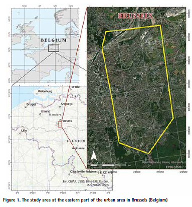
As the main goal of this study was to identify only the dominant urban tree species, all other non-dominant vegetations have been excluded during sampling. The sample plots were randomly selected, covering only the streets of the whole study area. Since in the parks most of the cases of tree crowns were overlapped and or completely overshadowed by the other species. That is why overcrowded tree populations were excluded to avoid misinterpretations of the species dominance information, during the final CS mapping. During field data collection, 75 plots (yellow dots in Figure 2) of 100 m2 (10 m × 10 m) each were selected throughout the study area following the well-known Simple Random Sampling (SRS) approach [79–82]. Only the areas with tree species dominance (i.e., woody or tall perennial plants) have been considered, excluding the ornamental herbs, shrubs, or grassland areas. The sample plots were also used during the training and validation of the tree species for GEOBIA classification. Among the 75 plots, 20 plots (red square boxes in Figure 2) were considered for the CS mapping and validation. The Diameter at Breast Height (DBH) was measured for each tree in the plot. The height (H) of trees was measured utilizing the hypsometer Nikon Forestry 550, a laser rangefinder with angle compensation technology optimized for forestry use [83], and a field computer was used to mark the plots on QGIS. Field data (H, DBH) were collected in the summer of 2019.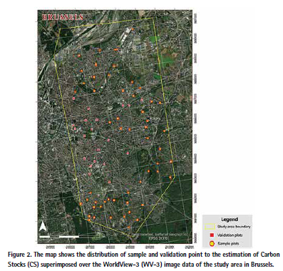
2.1.2. Remote Sensing Data
The airborne LiDAR dataset had been collected in Summer 2015 by Aerodata Surveys Nederland BV [84]. The Crown Height Model (CHM), i.e., the height of objects obtained through the difference between the digital surface model (DSM) and the digital terrain model (DTM), was produced at a spatial resolution of 0.25 m using the LAStools software [84].
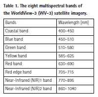
The WV3 image data for this study was acquired on 17 April 2017 (Figure 2), which provides one panchromatic band of 0.3 m and eight multispectral bands at 1.2 m spatial resolution (Table 1). The available WV-3 image data have been pan-sharpened at the initial stage. Pansharpening is the process of merging high-resolution panchromatic and multispectral imagery where the outcome is an image that has the high spectral resolution tion of the multispectral image and also the high spatial resolution of the panchromatic image [85–87].
The pan-sharpen process was conducted using the hyperspectral colour sharpening (HCS) algorithm that combines the high-resolution panchromatic data with lower res-olution multispectral data and specifically implemented for the WV imagery [88]. The cubic convolution resampling technique was chosen to resample the multispectral image to the high-resolution image using a 4 × 4 pixel moving window. The pan image and the multispectral image have been separately orthorectified using the DSM downloaded from the GeoPunt portal [89] and the available LiDAR data. All the steps were conducted in an ERDAS Imagine environment [90]. Later, the required shapefiles (for classification in Ecognition) were educed from the UrbIS database (UrbIS P& B and UrbIS-Adm), a general GIS database of the Brussels region [91].
2.2. Methodology
2.2.1. Geospatial Object-Based Image Analysis (GEOBIA) Classification
Tree species classification based on spectral properties is quite a matter of con-tention due to the high intra-class spectral heterogeneity and/or interclass spectral similarities [7,44,64–66]. The traditional pixel-based procedures, which classify each object only based on a distinct spectral signature (ignoring other spatial/contextual informa-tion) [48,92,93], are hardly capable of reaching an acceptable accuracy [94,95]. In our study, GEOBIA was applied, which is already approved as an efficient technique in the case of high-resolution image classifications [48,85,92,96– 99]. Instead of the single pixels, the GEOBIA approach typically works on: (i) Segmenting a remote sensing image into spectral similarities (i.e., segments or objects), and (ii) Evaluating the spectral, spatial, and/or context features of these segments for image classification [48,63,94,100,101]. As a result of segmentation, this approach can consider the textual and contextual information along with the spectral information during the classification [48,94,102– 104]. Therefore GEOBIA classification outcomes are more acceptable than those based on the existing traditional pixel-based approach [102,105–111]. .
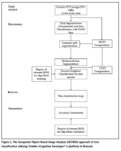
The Trimble eCognition Developer® 9 platform (Trimble, Munich, Germany) [112] was utilized to classify the dominant tree species in Brussels (Figure 3). At the initial stage, the chessboard segmentation has been introduced to initiate the GEOBIA classification approach. Then the primary classification was done utilizing the available shapefile from the Urbis database [91]. After that, the contrast split segmentation algorithm was implied to define the green and non-green areas with higher accuracy. This approach is based on the Normalized Difference Vegetation Index (NDVI) layer, where the ‘contrast split’ segments the scene into the dark and bright image objects based on a threshold value that maximizes the contrast between them [113]. The algorithm utilizes the optimal threshold separately for each image object which initiates a chessboard segmentation of variable scale and then performs the split on each square [114,115]. It was found quite helpful to identify the shadows, pathways, and pavements between the tree crowns.
Subsequently, the multiresolution segmentation (MRS) algorithm [116] was performed to group contiguous pixels into areas (i.e., segments) geometrically and radiometrically homogenous. The MRS algorithm was set by tuning the following parameters such as the “smoothness/ compactness” that determines the preferred shape of segments, and the “colour/ shape” parameter that controls the weights of spectral and shape information in the calculation of segments heterogeneity [48,94,117,118]. Considering the study of Choudhury et al. [36], green areas and streets have been identified with very large objects (as the size of the shapefile polygons) and have been classified separately from the rest. In these areas, a subsequent multiresolution segmentation had been applied to have the smaller objects. For this segmentation, rather than the thematic layers, the spectral information and the geometric information of WV-3 bands have been considered. The segmentation was done several times utilizing a different number of values for each parameter. For scale, the values were within 5 to 30, whereas for the shape and compactness, the values were between 0.1 to 0.9 [48,94,117,118]. After several attempts with different values, the ideal values utilized for segmentation, were found as scale parameter = 10, shape = 0.5 and the compactness = 0.8.
Before starting the Nearest Neighbour (NN) approach, an index known as Canopy Content Chlorophyll Index (CCCI) is used to separate the grasses from the vegetation class. This index can be calibrated as follows,
CCCI = NDRE/NDVI2
where, Normalized Difference Red Edge index [119]
NDRE = NIR2 – Red Edge/ NIR2 + Red Edge,
NDVI2 = NIR2 – Red/NIR2 + Red
Then the Nearest Neighbour (NN) algorithm [120] was performed, which is a supervised classification technique that classified all objects in the entire image based on the selected samples and the defined statistics [94]. For the sample selection and algorithm training, the sample plots had been considered. Once the algorithm training had been done, classification was initiated utilizing the “Assign class” algorithm. Three dominant tree species have been classified, such as Tilia spp. L., Acer spp. L. and Aesculus hippocastanum L. [121] covering the whole study area in Brussels. In this case, the larger and intensely green parks were not considered as it was hardly possible to differentiate crowns from a mixed or overlapped tree species population. Moreover, those trees could not be considered in further CS (AGB estimation) mapping due to the larger difference between the street and the park environment concerning tree health issues. Validation of the classification outcomes (Table 2) had also been done at the Trimble eCognition Developer® 9 platform [112] using confusion matrices [122–124] which is usually applied to compare the true classes with the ones assigned by the classifier on the generated maps. During the validation, 10%–15% of the total area for each class had been chosen as “true samples”, as known species or classes, to train the algorithm. The estimated producer accuracy shows the completeness of classification, and the user accuracy indicates the correctness of the classes [36,125], while the Hellden parameter is used to estimate the mean accuracy for each class. The mean accuracy for each class i can be calculated using the equation presented in [36,126]:
![]()
where A is the number of correctly classified reference points for class i, B is the total number of reference points in class i in the reference data, and C is the total number of reference points classified into class i.
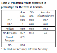
In Table 2, KIA known as Kappa Index of Agreement (or Cohen’s kappa coefficient), estimates the proportion of agreements [36,127]. Moreover, the overall accuracy (OA) has been estimated, which is the ratio of the sum of diagonal values of the confusion matrix to the total number of cell counts in the matrix [36,128].
2.2.2. Carbon Stock (CS) Mapping
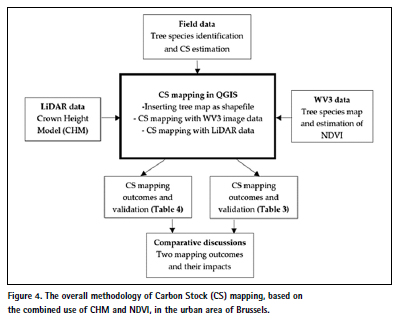
Several studies suggest that tree AGB is the most visible, dominant, dynamic, and essential pool of the terrestrial ecosystem [8,129–131], constituting around 30% of the total terrestrial ecosystem carbon pool [132]. In this study, based on the relationships among the WV-3 (NDVI) data and LiDAR (CHM) data derived variables and the field data, the predictive AGB estimation and, eventually, CS mapping has been done in both cases (Figure 4).
At first, the total AGB was calculated based on the field data (i.e., DBH, H, tree species, etc.) for each of the sample plots. For this calculation, an allometric model [133] was implied to calculate the AGB for each plot. The mean AGB/ plot estimation was necessaryas it is recommended that the tree above ground CS is assumed to be 50% of the total AGB [134–138]. Then to estimate the mean CS/plot, the mean AGB/plot was multiplied by 0.5 as a conversion factor [139–141]. Then in QGIS utilizing the WV-3 image data (from 2017, see Section 3.2.1 for details), the NDVI (Red edge and NIR1 band) of the whole study area was computed. The NDVI layer was considered in this study for the CS prediction and mapping, as previous studies claimed to find a strong correlation between the NDVI and total AGB of the trees [11,142–144]. In the case of LiDAR data, the CHM was utilized to map the CS for the dominant tree species. Then the NDVI-derived metrics were extracted for the sample plots utilizing the “Zonal statistics” plugin [145] at the QGIS interface. The CHM-derived matrices had been computed in the case of available LiDAR data (from 2015, see Section 3.2.2 for details). After that, the linear regression models were created in a Microsoft® Excel™ spreadsheet, calibrating the correlation between the mean CS/plot and the NDVI derived metrics to find out the best model to estimate and map the CS covering the whole study area [36]. The CHMderived matrices have also been done to determine the best model concerning the perspective CS mapping. A fishnet of 100 m2 (10 10 m) resolution (as for the sample plots) was built in QGIS for both cases (NDVI and CHM) to recognize the minimum to maximum CS zones, based on the dominant species map (exported as a shapefile in QGIS) obtained from the WV-3 image data. The classification shapefile was essential to define the regions of interest, providing QGIS to map the estimated CS values considering only the dominant tree species [36]. Otherwise, the map will show the CS values for other areas, i.e., the area covered with grass or even in an area where there is no vegetation.
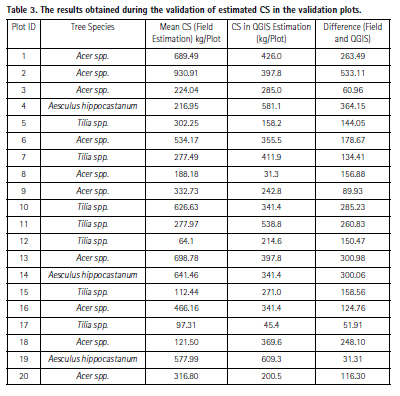
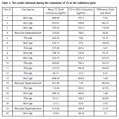
Then, to validate the mapping outcomes, 20 randomly selected plots have been utilized in both cases (NDVI and CHM).
This time the linear regression models were created only for the validation plots. Therefore, the differences (Tables 3 and 4) among the QGIS computed CS values, and the ground truth-values were shown to recognize the methodology’s effectiveness. The validation plots were the same in both cases, which was necessary to compare the impacts and to discuss the prospects and convenience of CS mapping in urban areas (see Section 4.2 for details).
References
1. 2014 Revision of the World Urbanization Prospects|Latest Major Publications—United Nations Department of Economic and Social Affairs. Available online: https://www.un.org/ en/development/desa/publications/2014- revision-world-urbanization-prospects. html (accessed on 5 May 2021).
2. Tzoulas, K.; Korpela, K.; Venn, S.; Yli-Pelkonen, V.; Ka´zmierczak, A.; Niemela, J.; James, P. Promoting ecosystem and human health in urban areas using Green Infrastructure: A literature review. Landsc. Urban Plan. 2007, 81, 167–178. [CrossRef]
3. de Vries, S.; van Dillen, S.M.; Groenewegen, P.P.; Spreeuwenberg, P. Streetscape greenery and health: Stress, social cohesion and physical activity as mediators. Soc. Sci. Med. 2013, 94, 26–33. [CrossRef] [PubMed]
4. Doick, K.J.; Davies, H.J.; Moss, J.; Coventry, R.; Handley, P.; Vazmonteiro, M.; Rogers, K.; Simpkin, P. The Canopy Cover of England’s Towns and Cities: Baselining and Setting Targets to Improve Human Health and Well-Being; University of Birmingham: Birmingham, UK, 2017; pp. 5–6.
5. Endreny, T.; Santagata, R.; Perna, A.; De Stefano, C.; Rallo, R.; Ulgiati, S. Implementing and managing urban forests: A much needed conservation strategy to increase ecosystem services and urban wellbeing. Ecol. Model. 2017, 360, 328–335. [CrossRef]
6. Nowak, D.J. Assessing Urban Forest Effects and Values: New York City’s Urban forest (Vol. 9); US Department of Agriculture, Forest Service, Northern Research Station: Madison, WI, USA, 2007.
7. Baines, O.; Wilkes, P.; Disney, M. Quantifying urban forest structure with open-access remote sensing data sets. Urban For. Urban Green. 2020, 50, 126653. [CrossRef]
8. Issa, S.; Dahy, B.; Ksiksi, T.; Saleous, N. A Review of Terrestrial Carbon Assessment Methods Using Geo-Spatial Technologies with Emphasis on Arid Lands. Remote Sens. 2020, 12, 2008. [CrossRef]
9. Jo, H.-K.; Kim, J.-Y.; Park, H.-M. Carbon reduction and planning strategies for urban parks in Seoul. Urban For. Urban Green. 2019, 41, 48–54. [CrossRef]
10. Behera, S.K.; Sahu, N.; Mishra, A.K.; Bargali, S.S.; Behera, M.D.; Tuli, R. Aboveground biomass and carbon stock assessment in Indian tropical deciduous forest and relationship with stand structural attributes. Ecol. Eng. 2017, 99, 513–524. [CrossRef]
11. Kanniah, K.D.; Muhamad, N.; Kang, C.S. Remote sensing assessment of carbon storage by urban forest. IOP Conf. Ser. Earth Environ. Sci. 2014, 18, 12151. [CrossRef]
12. Rosenfeld, A.H.; Akbari, H.; Romm, J.J.; Pomerantz, M. Cool communities: Strategies for heat island mitigation and smog reduction. Energy Build. 1998, 28, 51–62. [CrossRef]
13. Ferrini, F.; Fini, A. Sustainable Management Techniques for Trees in the Urban Areas. (2011): 1–19.
14. Steenberg, J.W.; Duinker, P.N.; Nitoslawski, S.A. Ecosystem-based management revisited: Updating the concepts for urban forests. Landsc. Urban Plan. 2019, 186, 24–35. [CrossRef]
15. Nitoslawski, S.A.; Galle, N.J.; Bosch, C.K.V.D.; Steenberg, J.W. Smarter ecosystems for smarter cities? A review of trends, technologies, and turning points for smart urban forestry. Sustain. Cities Soc. 2019, 51, 101770. [CrossRef]
16. Brack, C.L.; James, R.N.; Banks, J.C. Data Collection and Management for Tree Assets in Urban Environments. Proceeding Urban Data Management Symposium, 1999.
17. Brack, C. Pollution mitigation and carbon sequestration by an urban forest. Environ. Pollut. 2002, 116, S195–S200. [CrossRef]
18. Banks, J.; Brack, C.; James, R. Modelling changes in dimensions, health status, and arboricultural implications for urban trees. Urban Ecosyst. 1999, 3, 35–43. [CrossRef]
19. Nowak, D.J.; Crane, D.E. Carbon storage and sequestration by urban trees in the USA. Environ. Pollut. 2002, 116, 381–389.[CrossRef]
20. Nowak, D.J. Chicago’s Urban Forest Ecosystem: Results of the Chicago Urban Forest—E. Gregory McPherson—Google Books. Available online: https://books. google.it/books?hl=en&lr=&id=RnT26_ xGC-4C&oi=fnd&pg=PA83&ots=G9uEFur r1T&sig=4B7P3Onwpe9Qp84zgMYDsorM Viw&redir_esc=y#v=onepage&q&f=false (accessed on 9 January 2021).
21. Mokany, K.; Raison, R.J.; Prokushkin, A. Critical analysis of root: Shoot ratios in terrestrial biomes. Glob. Chang. Biol. 2005, 12, 84–96. [CrossRef]
22. Achard, F.; Eva, H.D.; Stibig, H.-J.; Mayaux, P.; Gallego, J.; Richards, T.; Malingreau, J.-P. Determination of Deforestation Rates of the World’s Humid Tropical Forests. Science 2002, 297, 999–1002. [CrossRef] [PubMed]
23. Brown, S. Estimating Biomass and Biomass Change of Tropical Forests: A Primer; Food & Agriculture Org.: Roma, Italy, 1997; Volume 134.
24. Liu, L.; Coops, N.C.; Aven, N.W.; Pang, Y. Mapping urban tree species using integrated airborne hyperspectral and LiDAR remote sensing data. Remote Sens. Environ. 2017, 200, 170–182. [CrossRef]
25. Dalponte, M.; Bruzzone, L.; Gianelle, D. Fusion of hyperspectral and LIDAR remote sensing data for classification of complex forest areas. IEEE Trans. Geosci. Remote Sens. 2008, 46, 1416–1427. [CrossRef]
26. Alonzo, M.; McFadden, J.P.; Nowak, D.J.; Roberts, D.A. Mapping urban forest structure and function using hyperspectral imagery and lidar data. Urban For. Urban Green. 2016, 17, 135–147. [CrossRef]
27. Zhang, Y.; Shen, W.; Li, M.; Lv, Y. Assessing spatio-temporal changes in forest cover and fragmentation under urban expansion in Nanjing, eastern China, from long-term Landsat observations (1987–2017). Appl. Geogr. 2020, 117, 102190. [CrossRef]
28. Zhang, M.; Du, H.; Mao, F.; Zhou, G.; Li, X.; Dong, L.; Zheng, J.; Zhu, D.; Liu, H.; Huang, Z.; et al. Spatiotemporal Evolution of Urban Expansion Using Landsat Time Series Data and Assessment of Its Influences on Forests. ISPRS Int. J. Geo. Inf. 2020, 9, 64.[CrossRef]
29. Shen, G.; Wang, Z.; Liu, C.; Han, Y. Mapping aboveground biomass and carbon in Shanghai’s urban forest using Landsat ETM+ and inventory data. Urban For. Urban Green. 2020, 51, 126655. [CrossRef]
30. Ren, Z.; Zheng, H.; He, X.; Zhang, D.; Yu, X.; Shen, G. Spatial estimation of urban forest structures with Landsat TM data and field measurements. Urban For. Urban Green. 2015, 14, 336–344. [CrossRef]
31. Moser, G.; Serpico, S.B.; Benediktsson, J.A. Land-cover mapping by Markov modeling of spatial–contextual information in very-high-resolution remote sensing images. Proc. IEEE 2012, 101, 631–651. [CrossRef]
32. Praticò, S.; Solano, F.; Di Fazio, S.; Modica, G. Machine Learning Classification of Mediterranean Forest Habitats in Google Earth Engine Based on Seasonal Sentinel-2 Time-Series and Input Image Composition Optimisation. Remote Sens. 2021, 13, 586.[CrossRef]
33. Fassnacht, F.E.; Latifi, H.; Stere ´nczak, K.; Modzelewska, A.; Lefsky, M.; Waser, L.; Straub, C.; Ghosh, A. Review of studies on tree species classification from remotely sensed data. Remote Sens. Environ. 2016, 186, 64–87. [CrossRef]
34. Van Ewijk, K.Y.; Randin, C.F.; Treitz, P.M.; Scott, N.A. Predicting fine-scale tree species abundance patterns using biotic variables derived from LiDAR and high spatial resolution imagery. Remote Sens. Environ. 2014, 150, 120–131. [CrossRef]
35. Chambers, D.; Périé, C.; Casajus, N.; De Blois, S. Challenges in modelling the abundance of 105 tree species in eastern North America using climate, edaphic, and topographic variables. For. Ecol. Manag. 2013, 291, 20–29. [CrossRef]
36. Choudhury, A.M.; Marcheggiani, E.; Despini, F.; Costanzini, S.; Rossi, P.; Galli, A.; Teggi, S. Urban Tree Species Identification and Carbon Stock Mapping for Urban Green Planning and Management. Forests 2020, 11, 1226. [CrossRef]
37. Vauhkonen, J.; Ørka, H.O.; Holmgren, J.; Dalponte, M.; Heinzel, J.; Koch, B. Tree Species Recognition Based on Airborne Laser Scanning and Complementary Data Sources; Springer: Berlin/Heidelberg, Germany, 2013; Volume 27, pp. 135–156.
38. Ørka, H.O.; Dalponte, M.; Gobakken, T.; Næsset, E.; Ene, L.T. Characterizing forest species composition using multiple remote sensing data sources and inventory approaches. Scand. J. For. Res. 2013, 28, 677–688. [CrossRef]
39. Adelabu, S.; Mutanga, O.; Adam, E.E.; Cho, M.A. Exploiting machine learning algorithms for tree species classification in a semiarid woodland using RapidEye image. J. Appl. Remote Sens. 2013, 7, 073480. [CrossRef]
40. Carleer, A.; Wolff, E. Exploitation of Very High Resolution Satellite Data for Tree Species Identification. Photogramm. Eng. Remote Sens. 2004, 70, 135–140. [CrossRef]
41. Ghosh, A.; Fassnacht, F.E.; Joshi, P.K.; Koch, B. A framework for mapping tree species combining hyperspectral and LiDAR data: Role of selected classifiers and sensor across three spatial scales. Int. J. Appl. Earth Obs. Geoinf. 2014, 26, 49–63. [CrossRef]
42. Jensen, R.R.; Hardin, P.J.; Hardin, A.J. Classification of urban tree species using hyperspectral imagery. Geocarto Int. 2012, 27, 443–458. [CrossRef]
43. Somers, B.; Asner, G.P. Tree species mapping in tropical forests using multi-temporal imaging spectroscopy: Wavelength adaptive spectral mixture analysis. Int. J. Appl. Earth Obs. Geoinf. 2014, 31, 57–66. [CrossRef]
44. Qian, Y.; Zhou, W.; Pickett, S.T.A.; Yu, W.; Xiong, D.; Wang, W.; Jing, C. Integrating structure and function: Mapping the hierarchical spatial heterogeneity of urban landscapes. Ecol. Process. 2020, 9, 1–11. [CrossRef]
45. Zhou, W.; Troy, A. An objectoriented approach for analysing and characterizing urban landscape at the parcel level. Int. J. Remote Sens. 2008, 29, 3119–3135. [CrossRef]
46. Ouma, Y.O.; Tateishi, R. Urbantrees extraction from Quickbird imagery using multiscale spectex-filtering and non-parametric classification. ISPRS J. Photogramm. Remote Sens. 2008, 63, 333–351. [CrossRef]
47. Lee, D.S.; Shan, J.; Bethel, J.S. Class-Guided Building Extraction from Ikonos Imagery. Photogramm. Eng. Remote Sens. 2003, 69, 143–150. [CrossRef]
48. Johnson, B.A.; Jozdani, S.E. Identifying Generalizable Image Segmentation Parameters for Urban Land Cover Mapping through Meta- Analysis and Regression Tree Modeling. Remote Sens. 2018, 10, 73. [CrossRef]
49. Degerickx, J.; Hermy, M.; Somers, B. Mapping Functional Urban Green Types Using High Resolution Remote Sensing Data. Sustainability 2020, 12, 2144. [CrossRef]
50. Puissant, A.; Rougier, S.; Stumpf, A. Object-oriented mapping of urban trees using Random Forest classifiers. Int. J. Appl. Earth Obs. Geoinf. 2014, 26, 235–245. [CrossRef]
51. Pu, R.; Landry, S. Mapping urban tree species by integrating multi-seasonal high resolution pléiades satellite imagery with airborne LiDAR data. Urban For. Urban Green. 2020, 53, 126675. [CrossRef]
52. Pu, R.; Landry, S. A comparative analysis of high spatial resolution IKONOS and WorldView-2 imagery for mapping urban tree species. Remote Sens. Environ. 2012, 124, 516–533. [CrossRef]
53. Mitchell, M.G.; Johansen, K.; Maron, M.; McAlpine, C.; Wu, D.; Rhodes, J.R. Identification of fine scale and landscape scale drivers of urban aboveground carbon stocks using high-resolution modeling and mapping. Sci. Total. Environ. 2018, 622- 623, 57–70.[CrossRef] [PubMed]
54. Caynes, R.J.C.; Mitchell, M.G.E.; Wu, D.S.; Johansen, K.; Rhodes, J.R. Using high-resolution LiDAR data to quantify the three-dimensional structure of vegetation in urban green space. Urban Ecosyst. 2016, 19, 1749–1765. [CrossRef]
55. Birdal, A.C.; Avdan, U.; Türk, T. Estimating tree heights with images from an unmanned aerial vehicle. Geomat. Nat. Hazards Risk 2017, 8, 1144–1156. [CrossRef]
56. Alonzo, M.; Bookhagen, B.; Roberts, D.A. Urban tree species mapping using hyperspectral and lidar data fusion. Remote Sens. Environ. 2014, 148, 70–83. [CrossRef]
57. Kim, S.; McGaughey, R.J.; Andersen, H.-E.; Schreuder, G. Tree species differentiation using intensity data derived from leaf-on and leaf-off airborne laser scanner data. Remote Sens. Environ. 2009, 113, 1575–1586. [CrossRef]
58. Plowright, A.A.; Coops, N.C.; Eskelson, B.N.; Sheppard, S.R.; Aven, N.W. Assessing urban tree condition using airborne light detection and ranging. Urban For. Urban Green. 2016, 19, 140–150. [CrossRef]
59. Kim, S.; Hinckley, T.; Briggs, D. Classifying individual tree genera using stepwise cluster analysis based on height and intensity metrics derived from airborne laser scanner data. Remote Sens. Environ. 2011, 115, 3329–3342. [CrossRef]
60. Ørka, H.O.; Næsset, E.; Bollandsås, O.M. Classifying species of individual trees by intensity and structure features derived from airborne laser scanner data. Remote Sens. Environ. 2009, 113, 1163–1174. [CrossRef]
61. Yao, W.; Krzystek, P.; Heurich, M. Tree species classification and estimation of stem volume and DBH based on single tree extraction by exploiting airborne full-waveform LiDAR data. Remote Sens. Environ. 2012, 123, 368–380. [CrossRef]
62. Myeong, S.; Nowak, D.J.; Hopkins, P.F.; Brock, R.H. Urban cover mapping using digital, highspatial resolution aerial imagery. Urban Ecosyst. 2001, 5, 243–256. [CrossRef]
63. Qian, Y.; Zhou, W.; Nytch, C.J.; Han, L.; Li, Z. A new index to differentiate tree and grass based on high resolution image and objectbased methods. Urban For. Urban Green. 2020, 53, 126661. [CrossRef]
64. Azeez, O.S.; Pradhan, B.; Shafri, H.Z.M.; Shukla, N.; Lee, C.H.; Rizeei, H.M. Modeling of CO emissions from traffic vehicles using artificial neural networks. Appl. Sci. 2019, 9, 313. [CrossRef]
65. Wilkes, P.; Disney, M.; Vicari, M.; Calders, K.; Burt, A. Estimating urban above ground biomass with multi-scale LiDAR. Carbon Balance Manag. 2018, 13, 10. [CrossRef]
66. Zhu, Z.; Zhou, Y.; Seto, K.C.; Stokes, E.C.; Deng, C.; Pickett, S.T.; Taubenböck, H. Understanding an urbanizing planet: Strategic directions for remote sensing. Remote Sens. Environ. 2019, 228, 164–182. [CrossRef]
67. Maynard, C.L.; Lawrence, R.L.; Nielsen, G.A.; Decker, G. Modeling Vegetation Amount Using Bandwise Regression and Ecological Site Descriptions as an Alternative to Vegetation Indices. GISci. Remote Sens. 2007, 44, 68–81. [CrossRef]
68. Kankare, V.; Vastaranta, M.; Holopainen, M.; Räty, M.; Yu, X.; Hyyppä, J.; Hyyppä, H.; Alho, P.; Viitala, R. Retrieval of Forest Aboveground Biomass and Stem Volume with Airborne Scanning LiDAR. Remote Sens. 2013, 5, 2257–2274. [CrossRef]
69. Wannasiri, W.; Nagai, M.; Honda, K.; Santitamnont, P.; Miphokasap, P. Extraction of Mangrove Biophysical Parameters Using Airborne LiDAR. Remote Sens. 2013, 5, 1787–1808. [CrossRef]
70. Lu, D. The potential and challenge of remote sensing-based biomass estimation. Int. J. Remote Sens. 2006, 27, 1297–1328. [CrossRef]
71. Foody, G.M.; Boyd, D.S.; Cutler, M. Predictive relations of tropical forest biomass from Landsat TM data and their transferability between regions. Remote Sens. Environ. 2003, 85, 463–474. [CrossRef]
72. Kobayashi, S.; Omura, Y.; Sanga-Ngoie, K.; Widyorini, R.; Kawai, S.; Supriadi, B.; Yamaguchi, Y. Characteristics of Decomposition Powers of L-Band Multi-Polarimetric SAR in Assessing Tree Growth of Industrial Plantation Forests in the Tropics. Remote Sens. 2012, 4, 3058–3077. [CrossRef]
73. Clewley, D.; Lucas, R.; Accad, A.; Armston, J.; Bowen, M.; Dwyer, J.; Pollock, S.; Bunting, P.; McAlpine, C.; Eyre, T.; et al. An Approach to Mapping Forest Growth Stages in Queensland, Australia through Integration of ALOS PALSAR and Landsat Sensor Data. Remote Sens. 2012, 4, 2236–2255. [CrossRef]
74. Robinson, C.; Saatchi, S.; Neumann, M.; Gillespie, T. Impacts of Spatial Variability on Aboveground Biomass Estimation from L- Band Radar in a Temperate Forest. Remote Sens. 2013, 5, 1001–1023. [CrossRef]
75. Zheng, D.; Rademacher, J.; Chen, J.; Crow, T.; Bresee, M.; Le Moine, J.; Ryu, S.-R. Estimating aboveground biomass using Landsat 7 ETM+ data across a managed landscape in northern Wisconsin, USA. Remote Sens. Environ. 2004, 93, 402–411. [CrossRef]
76. Coulibaly, L.; Migolet, P.; Adegbidi, H.; Fournier, R.; Hervet, E. Mapping Aboveground Forest Biomass from Ikonos Satellite Image and Multi-Source Geospatial Data using Neural Networks and a Kriging Interpolation. Int. Geosci. Remote Sens. Symp. 2008, 3, III-298. [CrossRef]
77. Castel, T. Retrieval biomass of a large Venezuelan pine plantation using JERS-1 SAR data. Analysis of forest structure impact on radar signature. Remote Sens. Environ. 2002, 79, 30–41. [CrossRef]
78. Wijaya, A.; Gloaguen, R. Fusion of ALOS Palsar and Landsat ETM data for land cover classification and biomass modeling using non-linear methods. Int. Geosci. Remote Sens. Symp. 2009, 3, III-581. [CrossRef]
79. Simple Random Sampling of Individual Items in the Absence of a Sampling Frame that Lists the Individuals|New Zealand Journal of Forestry Science|Full Text. Available online: https:// nzjforestryscience.springeropen.com/ articles/10.1186/s40490-016-0071- 1 (accessed on 24 May 2021).
80. West, P.W. Simple random sampling of individual items in the absence of a sampling frame that lists the individuals. N. Z. J. For. Sci. 2016, 46, 1–7. [CrossRef]
81. Gregoire, T.G.; Valentine, H.T. Sampling Strategies for Natural Resources and the Environment; Chapman and Hall/ CRC: Boca Raton, FL, USA, 2007.
82. Pinkham, R.S. An Efficient Algorithm for Drawing a Simple Random Sample. J. R. Stat. Soc. Ser. C Appl. Stat. 1987, 36, 370.[CrossRef]
83. Nikon|News|Nikon Introduces New Laser Rangefinder “Forestry 550”. Available online: https://www.nikon. com/news/2008 /0924_forestry_02.htm (accessed on 16 November 2020).
84. Degerickx, J.; Roberts, D.; McFadden, J.; Hermy, M.; Somers, B. Urban tree health assessment using airborne hyperspectral and LiDAR imagery. Int. J. Appl. Earth Obs. Geoinf. 2018, 73, 26–38. [CrossRef]
85. Solano, F.; Di Fazio, S.; Modica, G. A methodology based on GEOBIA and WorldView-3 imagery to derive vegetation indices at tree crown detail in olive orchards. Int. J. Appl. Earth Obs. Geoinf. 2019, 83, 101912. [CrossRef]
86. Gilbertson, J.K.; Kemp, J.; van Niekerk, A. Effect of pan-sharpening multi-temporal Landsat 8 imagery for crop type differentiation using different classification techniques. Comput. Electron. Agric. 2017, 134, 151–159. [CrossRef]
87. Karakus, P.; Karabork, H. Effect of pansharpened image on some of pixel based and object based classification accuracy. ISPRS Int. Arch. Photogramm. Remote Sens. Spat. Inf. Sci. 2016, XLI-B7, 235–239. [CrossRef]
88. Padwick, C.; Deskevich, M.; Pacifici, F.; Smallwood, S. WorldView-2 Pan-Sharpening. In Proceedings of the ASPRS 2010 Annual Conference, San Diego, CA, USA, 26–30 April 2010; Volume 2630, pp. 1–14.
89. Geopunt.be—The Flemish Geoportal|Con Terra. Available online: https://www.con-terra.com/ casestudies/geopuntbe-flemish-geoportal (accessed on 9 January 2021).
90. ERDAS IMAGINE: World-Class Remote Sensing Software|Hexagon Geospatial. Available online: https:// www.hexagongeospatial. com/products/ power-portfolio/erdas-imagine/erdasimagine- remote-sensing-softwarepackage (accessed on 9 January 2021).
91. UrbIS Download. Available online: http://urbisdownload.gis. irisnet.be/en/temporality/ (accessed on 16 November 2020).
92. Jebur, M.N.; Shafri, H.Z.M.; Pradhan, B.; Tehrany, M.S. Per-pixel and object-oriented classification methods for mapping urban land cover extraction using SPOT 5 imagery. Geocarto Int. 2013, 29, 792–806. [CrossRef]
93. Wang, L.; Sousa, W.P.; Gong, P. Integration of object-based and pixel-based classification for mapping mangroves with IKONOS imagery. Int. J. Remote Sens. 2004, 25, 5655–5668. [CrossRef]
94. Makinde, E.O.; Salami, A.; Olaleye, J.B.; Okewusi, O.C. Object Based and Pixel Based Classification Using Rapideye Satellite Imager of ETIOSA, Lagos, Nigeria. Geoinformatics FCE CTU 2016, 15, 59–70. [CrossRef]
95. Blaschke, T.; Lang, S.; Lorup, E.; Strobl, J.; Zeil, P. Object-oriented image processing in an integrated GIS/remote sensing environment and perspectives for environmental applications. Environ. Inf. Plan. Politics Public 2000, 2, 555–570.
96. Estoque, R.C.; Murayama, Y.; Akiyama, C. Pixel-based and object-based classifications using high- and medium-spatial-resolution imageries in the urban and suburban landscapes. Geocarto Int. 2015, 30, 1113–1129. [CrossRef]
97. Li, X.; Meng, Q.; Gu, X.; Jancsó, T.; Yu, T.; Wang, K.; Mavromatis, S. A hybrid method combining pixel-based and object-oriented methods and its application in Hungary using Chinese HJ-1 satellite images. Int. J. Remote Sens. 2013, 34, 4655–4668. [CrossRef]
98. Jabari, S.; Zhang, Y. Very High Resolution Satellite Image Classification Using Fuzzy Rule-Based Systems. Algorithms 2013, 6, 762–781. [CrossRef]
99. Platt, R.V.; Rapoza, L. An Evaluation of an Object-Oriented Paradigm for Land Use/Land Cover Classification*. Prof. Geogr. 2008, 60, 87–100. [CrossRef]
100. Wieland, M.; Pittore, M. Performance Evaluation of Machine Learning Algorithms for Urban Pattern Recognition from Multispectral Satellite Images. Remote Sens. 2014, 6, 2912–2939. [CrossRef]
101. Gao, Y.; Mas, J.F. 2008. A Comparison of the Performance of Pixel Based and Object Based Classifications over Images with Various Spatial Resolutions. Available online: https://medwelljournals.com/ abstract/?doi=ojesci.2008.27.35 (accessed on 24 May 2021).
102. Han, R.; Liu, P.; Wang, G.; Zhang, H.; Wu, X. Advantage of Combining OBIA and Classifier Ensemble Method for Very High-Resolution Satellite Imagery Classification. J. Sens. 2020, 2020, 1–15. [CrossRef]
103. Hossain, M.D.; Chen, D. Segmentation for Object-Based Image Analysis (OBIA): A review of algorithms and challenges from remote sensing perspective. ISPRS J. Photogramm. Remote Sens. 2019, 150, 115–134. [CrossRef]
104. Kucharczyk, M.; Hay, G.; Ghaffarian, S.; Hugenholtz, C. Geographic Object-Based Image Analysis: A Primer and Future Directions. Remote Sens. 2020, 12, 2012. [CrossRef]
105. Blaschke, T. Object based image analysis for remote sensing. ISPRS J. Photogramm. Remote Sens. 2010, 65, 2–16. [CrossRef]
106. Fu, B.; Wang, Y.; Campbell, A.; Li, Y.; Zhang, B.; Yin, S.; Xing, Z.; Jin, X. Comparison of object-based and pixel-based Random Forest algorithm for wetland vegetation mapping using high spatial resolution GF-1 and SAR data. Ecol. Indic. 2017, 73, 105–117.[CrossRef]
107. Duro, D.C.; Franklin, S.; Dubé, M.G. A comparison of pixel-based and object-based image analysis with selected machine learning algorithms for the classification of agricultural landscapes using SPOT-5 HRG imagery. Remote Sens. Environ. 2012, 118, 259–272.[CrossRef]
108. Myint, S.W.; Gober, P.; Brazel, A.; Grossman-Clarke, S.; Weng, Q. Per-pixel vs. object-based classification of urban land cover extraction using high spatial resolution imagery. Remote Sens. Environ. 2011, 115, 1145–1161. [CrossRef]
109. Martins, V.S.; Kaleita, A.L.; Gelder, B.K.; da Silveira, H.L.; Abe, C.A. Exploring multiscale object-based convolutional neural network (multi- OCNN) for remote sensing image classification at high spatial resolution. ISPRS J. Photogramm. Remote Sens. 2020, 168, 56–73. [CrossRef]
110. Su, T.; Liu, T.; Zhang, S.; Qu, Z.; Li, R. Machine learningassisted region merging for remote sensing image segmentation. ISPRS J. Photogramm. Remote Sens. 2020, 168, 89–123. [CrossRef]
111. De Pinho, C.M.D.; Fonseca, L.M.G.; Korting, T.S.; Almeida, C.; Kux, H.J.H. Land-cover classification of an intra-urban environment using high-resolution images and object-based image analysis. Int. J. Remote Sens. 2012, 33, 5973–5995. [CrossRef]
112. AGD. ECognition Version 5 Object Oriented Image Analysis User Guide; AGD: Munich, Germany, 2005.
113. Basic Rule Set Editing. Available online: https://docs. ecognition.com/v9.5.0/eCognition_ documentation/UserGuideDeveloper/ 4BasicRuleSetEditing.htm (accessed on 17 November 2020).
114. El-Naggar, A.M. Determination of optimum segmentation parameter values for extracting building from remote sensing images. Alex. Eng. J. 2018, 57, 3089–3097. [CrossRef]
115. Huang, J.; Zhang, X.; Xin, Q.; Sun, Y.; Zhang, P. Automatic building extraction from high-resolution aerial images and LiDAR data using gated residual refinement network. ISPRS J. Photogramm. Remote Sens. 2019, 151, 91–105. [CrossRef]
116. Multiresolution Segmentation: An Optimization Approach . . . / Multiresolution-Segmentation-An- Optimization-Approach.pdf/PDF4PRO. Available online: https://pdf4pro.com/ view/multiresolution-segmentationan- optimization-approach-598443. html (accessed on 19 May 2021).
117. Modica, G.; Messina, G.; De Luca, G.; Fiozzo, V.; Praticò, S. Monitoring the vegetation vigor in heterogeneous citrus and olive orchards. A multiscale object-based approach to extract trees’ crowns from UAV multispectral imagery. Comput. Electron. Agric. 2020, 175, 105500. [CrossRef]
118. Benz, U.C.; Hofmann, P.; Willhauck, G.; Lingenfelder, I.; Heynen, M. Multi-resolution, objectoriented fuzzy analysis of remote sensing data for GIS-ready information. ISPRS J. Photogramm. Remote Sens. 2004, 58, 239–258. [CrossRef]
119. Carneiro, F.M.; Furlani, C.E.A.; Zerbato, C.; De Menezes, P.C.; Gírio, L.A.D.S. Correlations among vegetation indices and peanut traits during different crop development stages. Eng. Agríc. 2019, 39, 33–40. [CrossRef]
120. Blanzieri, E.; Melgani, F. Nearest Neighbor Classification of Remote Sensing Images with the Maximal Margin Principle. IEEE Trans. Geosci. Remote Sens. 2008, 46, 1804–1811. [CrossRef]
121. Blunt, W. Linnaeus: The Compleat Naturalist; Princeton University Press: Princeton, NJ, USA, 2001; Available online: https: //www.worldcat.org/ title/linnaeus-the-compleat-naturalist/ oclc/1159631211?referer=di&ht=edition (accessed on 24 May 2021).
122. Gupta, D.L.; Malviya, A.K.; Singh, S. Performance Analysis of Classification Tree Learning Algorithms. Int. J. Comput. Appl. 2012, 55, 39–44. [CrossRef]
123. Immitzer, M.; Vuolo, F.; Atzberger, C. First Experience with Sentinel-2 Data for Crop and Tree Species Classifications in Central Europe. Remote Sens. 2016, 8, 166. [CrossRef]
124. So-In, C.; Mongkonchai, N.; Aimtongkham, P.; Wijitsopon, K.; Rujirakul, K. An evaluation of data mining classification models for network intrusion detection. In Proceedings of the 2014 Fourth International Conference on Digital Information and Communication Technology and its Applications (DICTAP), Bangkok, Thailand, 6–8 May 2014; pp. 90–94.
125. Foody, G.M. Assessing the Accuracy of Remotely Sensed Data: Principles and Practices. Photogramm. Rec. 2010, 25, 204–205.[CrossRef]
126. Helldén, U. A Test of Landsat-2 Imagery and Digital Data for Thematic Mapping Illustrated by an Environmental Study in Northern Kenya; Lund University: Lund, Sweden, 1980.
127. Cohen, J. Weighted kappa: Nominal scale agreement provision for scaled disagreement or partial credit. Psychol. Bull. 1968, 70, 213–220. [CrossRef] [PubMed]
128. Banko, G. A Review of Assessing the Accuracy of Classifications of Remotely Sensed Data and of Methods Including Remote Sensing Data in Forest Inventory; IIASA Interim Report; IIASA: Laxenburg, Austria, 1998; IR-98-081.
129. Gallaun, H.; Zanchi, G.; Nabuurs, G.J.; Hengeveld, G.; Schardt, M.; Verkerk, P.J. EU-wide maps of growing stock and above-ground biomass in forests based on remote sensing and field measurements. For. Ecol. Manag. 2010, 260, 252–261. [CrossRef]
130. Cairns, M.A.; Brown, S.; Helmer, E.H.; Baumgardner, G.A. Root biomass allocation in the world’s upland forests. Oecologia 1997, 111, 1–11. [CrossRef] [PubMed]
131. Fonton, N.H.; Medjibé, V.; Djomo, A.; Kondaoulé, J.; Rossi, V.; Ngomanda, A.; Maïdou, H. Analyzing Accuracy of the Power Functions for Modeling Aboveground Biomass Prediction in Congo Basin Tropical Forests. Open J. For. 2017, 07, 388–402.[CrossRef]
132. Kumar, L.; Sinha, P.; Taylor, S.; AlQurashi, A.F. Review of the use of remote sensing for biomass estimation to support renewable energy generation. J. Appl. Remote Sens. 2015, 9, 097696. [CrossRef]
133. Tabacchi, G.; Cosmo, D.; Gasparini, L. Aboveground tree volume and Phytomass Prediction Equations for Forest Species in Italy. Eur. J. For. Res. 2011, 130, 911–934. [CrossRef]
134. Goslee, K.; Walker, S.M.; Grais, A.; Murray, L.; Casarim, F.; Brown, S. Leaf Technicial Guidance Series for the Development of a Forest Carbon Monitoring System for REDD+: Module C-CS: Calculations for Estimating Carbon Stocks; Winrock International: Morrilton, AR, USA, 2010.
135. Biomass, B.S.E. And Biomass Change of Tropical Forests: A Primer. Rome FAO For. Pap. 1986, 134.
136. Losi, C.J.; Siccama, T.G.; Condit, R. Analysis of Alternative Methods for Estimating Carbon Stock in Young Tropical Plantatiions. For. Ecol. Manag. 2003, 184, 355–368. [CrossRef]
137. Vashum, K.T.; Jayakumar, S. Methods to Estimate Above- Ground Biomass and Carbon Stock in Natural Forests-a Review. J. Ecosyst. Ecography 2012, 2, 1–7. [CrossRef]
138. Whittaker, R.H. Carbon in the Biota. In Woodwell GM, Pecan EV, Carbon in the biosphere. In Proceedings of the 24th Brookhaven Symposium in Biology, New York, NY, USA, 16–18 May 1972; pp. 281–302.
139. Food and Agriculture Organization. Food and Agriculture Organization of the United Nations. Retrieved; Food and Agriculture Organization: Rome, Italy, 2010; p. 2012.
140. Vicharnakorn, P.; Shrestha, R.P.; Nagai, M.; Salam, A.P.; Kiratiprayoon, S. Carbon Stock Assessment Using Remote Sensing and Forest Inventory Data in Savannakhet, Lao PDR. Remote Sens. 2014, 6, 5452–5479. [CrossRef]
141. Panel, I. On Climate Change (IPCC); Cambridge University Press: Cambridge, UK, 2007.
142. Rahetlah, B.V.; Salgado, P.; Andrianarisoa, B.; Tillard, E.; Razafindrazaka, H.; Le Mezo, L.; Ramalanjaona, V.L. 2014. Relationship between Normalized Difference Vegetation Index (NDVI) and Forage Biomass Yield in the Vakinankaratra Region, Madagascar.
143. Goswami, S.; Gamon, J.; Vargas, S.; Tweedie, C. Relationships of NDVI, Biomass, and Leaf Area Index (LAI) for Six Key Plant Species in Barrow, Alaska. PeerJ Prepr. 2015, 19.
144. Coelho, A.P.; Rosalen, D.L.; De Faria, R.T. Vegetation indices in the prediction of biomass and grain yield of white oat under irrigation levels. Pesquisa Agropecuária Tropical 2018, 48, 109–117. [CrossRef]
145. Jung, M. 2013. LecoS-A QGIS plugin for automated landscape ecology analysis (No. e116v2). PeerJ 2013. [CrossRef]
Copyright: © 2021 by the authors. Licensee MDPI, Basel, Switzerland. This article is an open access article distributed under the terms and conditions of the Creative Commons Attribution (CC BY) license (https:// creativecommons.org/licenses/by/ 4.0/)
The paper originally published in Forests 2021, 12,692. https://doi. org/10.3390/ f12060692 has been republished wth authors’ permission.
To be concluded in the next issue.


 (3 votes, average: 4.00 out of 5)


Leave your response!