| Mapping | |
Effect of GCPs in distribution and location on geometric correction of corona satellite image
This paper deals with geometric correction of CORONA satellite image which make use of non-parametric approach. |
 |
|
 |
|
Digital images collected form airborne or space-borne sensors often contain systematic and non-systematic geometric errors that arises from the earth curvature, platform motion, relief displacement, nonlinearities in scanning motion, the earth rotation, etc . [1]. The intent of geometric correction is to compensate for the distortions introduced by these factors so that the correct image will have the highest practical geometric integrity.
The geometric correction process is normally implemented as a two-step procedure. First, those distortions that are systematic, or predictable, are considered. Second, those distortions that are essentially random, or unpredictable, are considered.
Systematic distortions are well understood and easily corrected by applying formulas derived by modeling the sources of the distortions mathematically. Random distortions and residual unknown systematic distortions are corrected by analyzing well-distributed ground control points (GCPs) occurring in an image. In the correction process numerous GCPs are located both in terms of their two image coordinates (column, row numbers) on the distorted image and in terms of their ground coordinates (typically measured from a map, or GPS located in the field, in terms of UTM coordinates or latitude and longitude). These values are then submitted to a least squares regression analysis to determine coefficients for two coordinate transformation equations that can be used to interrelate the geometrically correct (map) coordinates and the distorted-image coordinates.
After producing the transformation function, a processing called resampling is used to determine the pixel values to fill into the out matrix from the original image matrix. The process is performed using the following operations.
1. The coordinate of each element in the undistorted output matrix are transformed to determine their corresponding location in the original input (distorted-image) matrix.
2. In general, a cell in the output matrix will not directly overlay a pixel in the input matrix. Accordingly, the intensity value or digital number (DN) eventually assigned to a cell in the output matrix is determined on the basis of the pixel values that surround its transformed position in the original output input matrix [4].
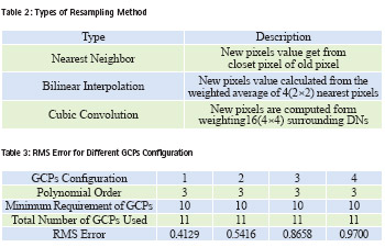
Commonly used methods for resampling are nearest neighbor, bilinear interpolation, and cubic convolution.
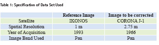
Study area and data set used
The reference image which is already geometrically corrected was acquired in 1993 by IKONOS comprising the region of Yangon, Myanmar. The image to be geometrically corrected was acquired in 1966 by CORONA that captured the same region as reference image.
Geometric correction
There are four different levels of geometric correction of remotely sensed imagery.
(a) Registration- alignment of one image to another image of the same area.
(b) Rectification- alignment of image to a map so that the image is planimetric, just like the map; also known as geo-referencing.
(c) Geocoding- A special case of rectification that includes scaling to a uniform standard pixel GIS.
(d) Orthorectification- Correction of the image, pixel by pixel for topographic distortion [2]
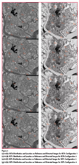
Image rectification is carried out in this work that is CORONA image of Yangon region is rectified to a georeferenced IKONOS image which has UTM coordinate using ERDAS IMAGINE software. The following GCPs configurations are considered.
Configuration 1: GCPs are well-distributed and their corresponding locations are easily identifiable in both images.
Configuration 2: GCPs are not welldistributed, but their corresponding locations are easily identifiable in both images.
Configuration 3: GCPs are welldistributed, but their corresponding locations are not easily identifiable in both images.
Configuration 4: GCPs are not well-distributed and their corresponding locations are not easily identifiable in both images.
For GCPs configurations 1 and 2, control points are carefully chosen because the acquisition time between the two images is too high. Theses control points are place at the places where it doesn’t change over time.
Polynomial Equation
A polynomial is a mathematical expression consisting of variables and coefficients. A coefficient is a constant, which is multiplied by a variable in the expression. The variables in polynomial expressions can be raised to exponents. The highest exponent in a polynomial determines the order of the polynomial. A polynomial with one variable, x, takes the following form:
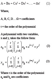
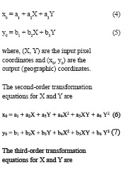
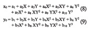
The following first-order polynomial transformation equations can be used to determine the coefficient required to transform pixel coordinate measurements to the corresponding other coordinate values.
The number of control points should be more than the number of unknown parameters in polynomial equations, because the errors are adjusted by the least-square method. The number of unknown parameters in polynomial transformation equation can be obtained using the following equation
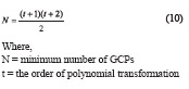
Depending on the geometric distortions, the order of polynomial is determined. Usually a maximum of third-order polynomial is sufficient for existing remote sensing images [1].
As the image to be rectified is highly distorted, third order polynomial transformation is chosen in this work. Based on equation (10), minimum numbers of GCPs should be at least 10 GCPs. Total number of GCPs chosen for this work is eleven.
Interpolation
Once applying geometric transformation, image may be shear, rotate, transformed or skewed. Pixel interpolation is necessary for filling missing values of area. For that pixel brightness values must be determined. There may not be any direct one-to-one relation between base image and image which is rectified. There is mechanism for determining the brightness value, this process is known as pixel interpolation.
Resampling
Resampling process used to determine the digital values to place in the new pixel location of the corrected output image, this process known as a resampling. Resampling required to estimate a new pixel between existing pixels due to non-integer transformed (x, y) . Table 2 shows types of resampling method [2] .
RMS Error
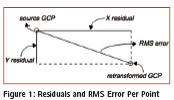
RMS error is the distance between the input (source) location of a GCP and the retransformed location for the same GCP. In other words, it is the difference between the desired output coordinate for a GCP and the actual output coordinate for the same point, when the point is transformed with the geometric transformation.
RMS error is calculated with a distance equation:
![]()
Where, xi and yi are the input (source) coordinates, and xr and yr are the retransformed coordinates RMS error is expressed as a distance in the source coordinate system. If data file coordinates are the source coordinates, then the RMS error is a distance in pixel widths. For example, an RMS error of 2 means that the reference pixel is 2 pixels away from the retransformed pixel.
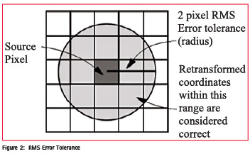
Tolerance of RMS Error
The amount of RMS error that is tolerated can be thought of as a window around each source coordinate, inside which a retransformed coordinate is considered to be correct (that is, close enough to use). For example, if the RMS error tolerance is 2, then the retransformed pixel can be 2 pixels away from the source pixel and still be considered accurate [3].
Experimental result
Table 3 shows the result on geometric correction using third order polynomial with different GCPs distribution and location.
Discussion and conclusion
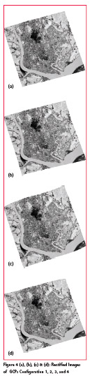
In this work, image to map geometric rectification of distorted image is performed based on third order polynomial. Rectification is carried out by four types of ground control points configuration in such a way that the impact on different distribution patterns of ground control points and their corresponding location is analyzed.
The first GCPs configuration is that GCPs are located at the places where they are easily and accurately identifiable in both images and their distribution is even across the image.
The second GCPs configuration is that GCPs are put at the points which are distinct, but they are not well distri buted across the image.
The third GCPs configuration is that GCPs distribution pattern is uniform across the image but they are not accurately identifiable.
The last GCPs configuration is that GCPs are not well distributed and their corresponding locations are not distinct.
Finally, the results on geometric rectification are evaluated by using the total root mean square error (RMSE). Based on the result, it shows that RMSE is the lowest in the case where GCPs distribution pattern is uniform across the image and their locations are at road intersection, building corner, and distinct natural features. RMSE is getting higher on GCPs configuration two to four by order. The worst case is that RMSE is the highest where GCPs distribution pattern are not evenly spread across on both images and their corresponding locations are not distinct.
In conclusion, based on experimental result, geometric correction accuracy of distorted image depends not only on the location of GCPs where they are placed at easily identifiable places (building corner, road intersection, etc.), but also on their distribution (evenly spread across the image).
References
[1] Bhatta. B., 2008. Remote Sensing and Gis. Oxford University, India, pp. 317-616.
[2] Chintan . D ., Rahul . J., Srivastava. S., 2015. A Survey on geometric correction of satellite imagery. International journal of computer applications, Vol 116 – No.12.
[3] Erdas, Inc. 1999. Erdas Field Guide, Retrieved August 30, 2016, from www. gis. us u.edu/ manuals/ labbook/ erdas/ manuals.
[4] Thomas. L., Ralph . K., Jonathan , C., Remote Sensing and Image Interpretation. Wiley, India, pp. 495.
The paper was presented at Asian Conference on Remote Sensing (ACRS), Colombo, Sri Lanka 17-21 October 2016


 (No Ratings Yet)


Leave your response!