| Application - New | |
Assessing the Quality of an UAV-based Orthomosaic and Surface Model of a Breakwater
This paper describes the conditions of the UAV flight and of the breakwater environment, conditions that were particularly hard, and presents the results of the quality control of the surface model made with the use of statistical methods |
 |
|
 |
|
 |
|
 |
|
 |
|
The breakwaters are built to protect infrastructure of ports. They are conceived and designed to withstand the most adverse and extreme weather conditions. The sea waves, the tides, the currents, winds, dynamics of underwater sediments and activities of the port, are some of the factors that lead to the degradation of breakwaters, and may restrict the activity of the port. One of the most insidious degradation is the removal of support materials that takes place beneath the blocks of protection on the surface. Quite often it is a localized process with slow progression and small effects on the surface of the breakwater, but that can be due to a major failure of a stretch of the structure and reduction of the functionality of the port.
When compared with structures like dams, bridges or large buildings, breakwaters are the structures much less monitored. As the deterioration of breakwaters usually doesn’t put lives in danger and usually large structural modifications are a consequence of big storms that hit coastal areas, very few breakwaters are regularly monitored.
The monitoring of a breakwater, particularly the measurement of displacements, faces big challenges that have, in many cases, weak solutions. Marujo et al. (2013) has made a survey of the different monitoring techniques (expert judgment techniques and quantitative/ automated techniques) available to monitor maritime and coastal structures. These include visual inspections (walking, waterborne, airborne, diving), closeup photography (terrestrial, waterborne, aerial and airborne), photogrammetry, videogrammetry, aerial photography (with normal or with unmanned aerial vehicles (UAV)), ‘crane and ball’ survey, topographic survey techniques (traditional and GNSS), multibeam and side scan sonar, Lidar, satellite images, InSAR methods and laser scanning.
Especially in breakwaters that protect small ports which don’t generate large incomes, the monitoring displacements with aerial photography taken by a digital camera mounted on an UAV should be tested because, as being an inexpensive technique, it can represent an interesting alternative to other methods. This paper describes the first stage of a test, which is undergone, on the use of UAV techniques to monitor the displacements of the breakwater of Ericeira, a structure exposed to the northwest Atlantic waves. Since its rebuilt in the 2010s, this breakwater has been used to test new methodologies of monitoring like the use of 3D laser, multibeam techniques and UAV-based generation of surface model. This last one is the object of the studies performed by the authors of this paper, that deals with the assessment of the quality of an orthomosaic and of the surface model based in photos taken from an UAV, during a flight that faced difficult conditions, also reported in this paper.
The breakwater of Ericeira
Ericeira is a seaside resort, 35 km northwest of Lisbon, capital of Portugal, where fishing continues to play an important role in the local economy. In the past few years, Ericeira area has seen growing in its importance as a leisure resort due to the large number of quality surf breaks, seven, in just 4 km of coastline.
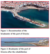
The port of Ericeira is mostly used by the local fisherman community. The advanced deterioration of the original protection of the quay (built in 1970s) was a consequence of the effect of the highly energetic north-westerly Atlantic Ocean waves on a under-dimensioned breakwater. A comprehensive study made by the National Laboratory for Civil Engineering (LNEC) in 2000, focused on the analysis of the status of pier under the perspective of its reconstruction and development of the port. The first stage of rehabilitation is already completed (Figures 1 and 2) and focused on rebuilding the breakwater and constructing new areas and buildings to support fishing activity.
The new rubble mound breakwater (RMB), which is longer and stronger, has created a wider area of sufficiently calm waters to allow safe operations of berthing, cargo transfer, vessels manoeuvre and protection of port infrastructures. The breakwater is 440 m long and 35 m wide. It consists of two straight lengths, angled at 147º to each other. The crest is 6.5 m wide and has an altitude of 9 m (referred to the hydrographic zero). The main elements of this breakwater are a core of finer material covered by big blocks (armor layer). Beneath the armor layer, a filter layer has been placed which is known as the underlayer, to prevent the finer material from being washed out through the armor layer.
Along the entire crest and on half of the leeside are two superstructures in concrete, being that the lowest one includes a quay. The most exposed slope of the breakwater (facing the northwesterly waves) is covered with tetrapods; the southwest extremity, which has a small lighthouse on the top, is covered with grooved cubes; the remaining areas are covered with large stones.
The UAV flight
The flight of the UAV airplane took place on February 9, 2013, after being delayed by a day due to strong winds in the area. It had to be carried out during high tide, not the best period of the day since many blocks were covered with water. The mix of these conditions (strong waves, wind, and high tide) made it impossible to find a good take-off/landing area nearby the breakwater. Ericeira village, on the top of the cliff that surrounds the port (see Figure 1), with a tight urban fabric, has no good areas either. The best one, a flat field with ground vegetation and no trees or bushes, was in the surroundings of Ericeira, nearly 1,200 m away from the port. It is necessary to state that this area was also chosen due to a clear sight to the area where the plane was going to operate in. On the slope between the take-off field (with at an elevation of about 100 m) and the port, there are several high buildings. For security reason, the altitude of the flight could not be set to a low value.
The photos were taken by a digital camera Canon IXUS 220 HS (3000×4000 pixels), mounted on the platform SenseFly Swinglet CAM (Figure 3), a very light (500 g) and small (80 cm wingspan) plane. The emission of data like battery level, speed of the wind, position of the UAV and a transmission that was made every 0.25 s to a control unit on land, would allow the monitoring of the flight. The control unit consists of the software eMotion (from Sensefly), installed on a laptop. This has an external radio antenna for communication. A more comprehensive description of the system can be found in Vallet et al. (2011).
EMotion was also used to programme the flight: To set the route, establish the height of the flight above ground, and to choose the points/area where to trigger the photos. In the flight above Ericeira breakwater, the following were set: i) the ground resolution, of 2 cm by pixel, ii) the area that needed to be covered, on a satellite view of the area downloaded from the internet, iii) the lateral overlap of the photos of 60%, iv) the longitudinal overlap of 90%. With this information, the software established automatically the flight eight (85 m), path (in the form of waypoints) and time interval between photos (a photo every two seconds). The flight plan was done at the office and transmitted to the airplane just before the flight. As explained before, it was impossible to find a good takeoff area near the breakwater being that since the location chosen had a height of 100 m. For this reason, the flight over the breakwater was done at an altitude of 185 m. As there is a strong connection between ground resolution and quality (Küng et al., 2011), the orthomosaic and the digital surface model generated from the photographs will have lower accuracy than initially expected.
During the flight there were problems with the transmission of data so the ground station received very few records from the airplane. When the UAV was over the breakwater, the ground station only received about 2% of the data expected, data that would have allowed to set an estimate on the location of the airplane (latitude, longitude, altitude), its attitude, speed, etc.
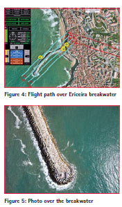
But, despite the communication problems and because the plane is completely autonomous, the flight was completed. The origin of these problems of communication might be related with radio interference caused by nearby communications antennae. Just before the flight over the breakwater it was performed another flight, 3 km southeast Ericeira, over a valley only with agricultural use. In this flight the only communication problems occurred when the airplane was behind hills and there was no line of sight to it. In Figure 4 we draw, on a GoogleMaps image, the programmed path of the flight (cyan lines) and the location of the centre of photographs (yellow dots), as received at the control station. From the 75 photographs taken, the ground station only received information about the flight in three of these. Figure 5 presents one of the photos taken.
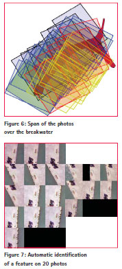
Despite the bad conditions of the flight, with high northeast winds, we got a good coverage of the breakwater, as seen in Figure 6 where we represented, over the orthomosaic of the breakwater, the approximate span of each photo on the ground (in this study, only the breakwater area was considered).
During the flight the wind direction, and velocity, were not constant but the predominance was NW-SE direction. During the second and forth strips (blue and yellow polygons in Figure 6) the airplane flew in the NE direction, against the wind. One can see that its velocity slowed down because it took more photos. One can also see that it was at the beginning of the survey (black polygons) that the wind presented more variations. Each spot of the breakwater was covered by at least five photos, being that some features are identified in 21 photos (see example in Figure 7 of a feature that can be seen in 20 photos).
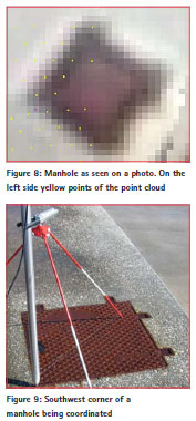
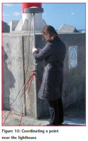
We determined the coordinates of several points (ground control points, GCP) of the superstructure of breakwater (Figure 11) by GNSS to reference the orthomosaic and the surface model and to assess planimetric and altimetric positional quality. We chose points that could be easily identified on the images (Figure 8), like the corners of the several square manhole covers placed along the superstructure (Figure 9), or the corners of the concrete base of the lighthouse (Figure 10). The points were coordinated using two Topcon choke ring antennae: one was placed on a tripod on the breakwater (reference station) and remained there during the surveying; the other was placed on top of a stick and on each point for three minutes. GNSS data was recorded at a period of 1 second. We calculated geodetic coordinates, in the ETRS89 reference frame, and cartographic coordinates, in the national coordinate system PT-TM06, using the software Pinacle and GNSS data of the nearest station of the Portuguese CORS Network.
Data processing
Despite the lack of information about the flight, the processing software PostFlight Terra 3D V1, also from Sensefly, was able to produce the orthomosaic and digital surface model.
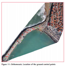
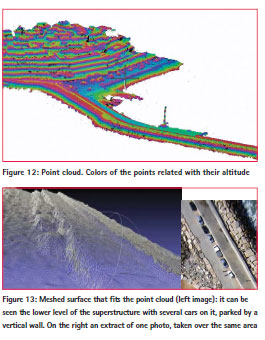
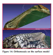
The orthomosaic (Figure 11) is an orthogonal projection of the ground from which it is possibly to get only planimetric coordinates. It is the result of the combination of two photogrammetric processing tools: ortho-rectification (correcting imagery for distortion induced by elevation using elevation data and camera model information) and mosaicking (process of taking two or more separate images and ‘stitching’ them together into a single image). Information about height is necessary to build the digital surface model, which was derived from a point cloud also generated by the same software. The surface is described by a set of discrete points, independent of each other. Each one has only three attributes – the three coordinates. In Figure 12, we present the point cloud (perspective of the breakwater) where we assigned a color to each point based on its altitude. In this phase, for visualization purposes, we generated a triangle mesh from the point cloud (Figure 13).
Both products, generated only with very few data available from the flight, had large errors (almost 116 m in planimetry, in the south extremity of the breakwater), so we had to use some of the GCP to georeference the breakwater. We chose five points (green dots in Figure 11): one point near land, another near the end of the breakwater and two in the middle.
Such a large difference that is unusual in UAV orthomosaics, is the result of: i) lack of information about majority of the photos (coordinates of the centre of projection of the photos and airplane orientation); ii) in many photos the majority of the pixels has information about the water and this can’t be used to stitch photos because it is impossible to find tie points; iii) small areas with tie points: the breakwater is a long and narrow structure that occupies a small area in each photo (photo in Figure 5 is a good example); iv) long areas with similar elements (monotonous tetrapods and stone blocks along a concrete strip). To surpass the problem, the only way was, as explained, to use some of the GCP as reference points. The points that we didn’t use as reference points were used to assess the quality of the orthomosaic and of the surface model. In the next paragraph, the tests will be presented, and the following paragraph will include the data used and the results of the tests.
Statistics to test the differences of coordinates
We applied statistical tests to assess the quality of orthomosaic and surface model, tests that are usually used to evaluate the positional quality (Casaca 1999, Morrison 1990). We tested the accuracy and precision of the data. The data used are differences between GNSS and photogrammetric coordinates of the GCP. The GNSS coordinates, estimated with an error smaller than 1 cm, are more accurate than the photogrammetric coordinates obtained from the orthomosaic and the surface model, and therefore, will be considered as reference coordinates.
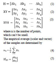
Let H (1,n), XY (2,n) and XYH (3,n) be matrices of the differences Δ between photogrammetric and GNSS coordinates:
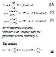
is distributed as a random variable chi-square, with the parameter of non-centrality ω.
Testing the Accuracy
We characterize the accuracy of the photogrammetric coordinates by testing the centrality of the distribution of the positional errors of these coordinates. Under the null hypothesis (H0), the scalar v, from (15), (16) or (17) has a Snedecor’s F distribution with f1 and f2 degrees of freedom; under the alternative hypothesis (HA), the scalar v has a non-central F distribution:
![]()
with f1=1, 2 or 3 when it is tested, respectively, altimetric, planimetric or 3D data. The degree of freedom f2 is equal to n-1. ω is a positive non-centrality parameter.
To test the null hypothesis against the alternative hypothesis, the variable of the test (v) is compared to the acceptance (RA) and critical (RC) regions:
![]()
where q is the 0.95 quantile of the Snedecor’s F distribution with f1 and f2 degrees of freedom.
Testing the Precision
We characterized the precision of the photogrammetric coordinates by testing the dispersion of the distribution of the positional errors of these coordinates. This test will allow us to assess if the orthomosaic/surface model is included in a pre-defined class of precision, class characterized by a tolerance (tJ), with a level of quality acceptable of, for instance, 0.95.
The variance σJ 2 of each class “J” of precision is determined by the following expression:
![]()
where q is the 0.95 quantile of the chisquared distribution with 1, 2 or 3 degrees of freedom, depending on the coordinates (1D, 2D or 3D) being tested.
For instance, if it is considered three classes (J=I, II or III) with tolerances tI=5 cm, tII=10 cm; tIII = 15cm, the values of variances of each class when testing planimetric coordinates, would be σI 2=4.17 cm2, σII 2=16.69 cm2, σIII 2=37.56 cm2, since q=5.99.
In this test each component, X, Y and H are analysed in an independent way. Under the null hypothesis, the scalar u, from (18) has a chi-squared distribution with (n-1) degrees of freedom; under the alternative hypothesis, u has a noncentral chi-squared distribution:
![]()
where ω is a positive non-centrality parameter. In equation (18), will be replaced by σJ 2, from the expression (21). The test will be performed as many times as the number of classes of precision established.
To test the null hypothesis against the alternative hypothesis, the variable of the test (u) is compared to the acceptance (RA) and critical (RC) regions:
![]()
where q is the 0.95 quantile of the qui-squared distribution with (n-1) degrees of freedom.
It was tested if each component was included in a chosen class of precision. To perform an analysis of the planimetric coordinates together (X and Y, as a whole) we will use a methodology adapted from the one presented by Mailing (1989). We will use a comparison of the ellipses with equal density of probability of the distribution of the planimetric inconsistencies with the corresponding circles of the planimetric tolerance. This test can be adapted to test the 3D coordinates.
Let λ be the smallest eigenvalue of the matrix of variance-covariance Σ-1, matrix which is unknown. The condition
![]()
is necessary and sufficient for, given a probability level (1-α), the corresponding ellipse with equal probability density lies inside the circle of tolerance with radius:
![]()
where q is the probability quantile (1 – α) of a central chi-square distribution. It has two degrees of freedom when testing planimetric coordinates; three when testing 3D coordinates. Usually α=0.05.
According to Morrison (1990), the largest and the smallest eigenvalues of the matrix S-1 in the planimetric case (2×2 matrix) are
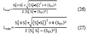
Knowing these eigenvalues is possible to build λ*, an estimator of the smallest (λ) eigenvalue of the matrix Σ-1 and calculate the statistics w and the maximum likelihood estimator of λ.
![]()
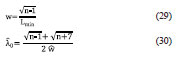
The estimates (27), (28) and (30) of the smallest eigenvalue λ can be used in the equation (24) to analyse if the level of tolerance can be accepted.
Results of applying the tests on the data
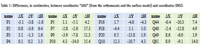
Ten points were used to assess the quality of the orthomosaic and the surface model. The planimetric coordinates were obtained from the orthomosaic using the software ArcGIS: the points were identified on the image and marked by a point. The attribute ‘planimetric coordinate’ of these points were transferred automatically to a text file. The height of these pointswere interpolated from the 2D barycentric coordinates. The differences between photogrammetric ‘UAV’ and GNSS coordinates are presented in Table 1.
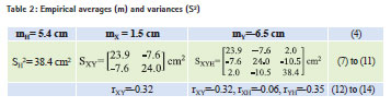
The next step of the evaluation is to determine the empirical averages and variances (see values in Table 2).
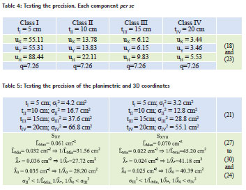
With these values, we were able to perform the calculus of: i) statistics vH, vXY and vXYH, and also of the statistics vX and vY (Table 3) to test the accuracy, ii) statistics u and the eigenvalues of matrices to test the precision (Tables 4 and 5).
When v ≤q, the distribution of errors is central. In Table 3, it can be seen that only the positional errors of the X component have a central distribution. This is not a surprise after a simple analysis of the values of Table 1, where it can be seen that the majority of the differences of the components Y and H have the same sign.
According to the data presented in Table 4, the orthomosaic can be included in class III of dispersion because both statistics (uX and uY) are smaller than q (the 0.95 quantile of the central chisquare distribution with 15 degrees of freedom). The component altitude, if considered independent, is classified as belonging to the class IV of dispersion.
To determine the eigenvalues of the matrix SXYH, it was used the Excel addin Matrix.
To set the class of dispersion of the planimetric coordinates and of the 3D coordinates, it was used the three estimators of λ presented at the end of the last paragraph. In the last line of Table 5, the values presented are calculated for these three estimators. According to these and the classes chosen, the orthomosaic belongs to class III of tolerance; the surface model (that gathers planimetric coordinates with altitude) belongs to class IV of dispersion.
Conclusions
Several tests were presented that could be used to assess the positional quality in products used to represent the surface of the Earth. It was applied to analyse the quality of an orthomosaic and a surface model produced from photos of a breakwater. The photos were taken by a common digital camera mounted on an UAV airplane. The flight was done under bad conditions: strong wind, unknown position and attitude of the airplane due to the lack of communications.
The root mean square error of the photogrammetric ‘UAV’ coordinates is 10 cm in planimetry and 8 cm in height. The tests performed indicate that accuracy was not achieved while concerning the precision the orthomosaic that lies in Class III (15 cm) and the surface model in Class IV (20 cm). These values are worse than the ones obtained from a very recent flight made with the same equipment over an area of 13.2 ha (the breakwater flight covered an area of 9.5 ha). In this larger area, in a city, it was possible to choose reference and control points all over it. Here, we were not limited to a narrow strip as in the breakwater study. Maybe this was the main reason for the achievement of better results.
References
Casaca,J. 1999. A Avaliação da Qualidade Posicional de Cartografia Topográfica em Escalas Grandes. Atas da II Conferência Nacional de Cartografia e Geodesia.
Küng, O., Strecha, C., Beyeler, A., Zufferey, J.C., Floreano, D., Fua, P., Gervaix, F. 2011. The accuracy of automatic photogrammetric techniques on ultra-light UAV imagery, Int. Arch. Photogramm. Remote Sens. Spatial Inf. Sci., XXXVIII-1/C22, 125-130, doi:10.5194/isprsarchives- XXXVIII-1-C22-125-2011.
Mailing, D. 1989. Elements of Cartometry. Pergamon Press.
Marujo,N., Trigo-Teixeira,A., Sanches do Valle,A., Araújo,M.A., Caldeira,J. 2013. An improved and integrated monitoring methodology for rubble mound breakwaters – application to the Ericeira breakwater. 6th SCACR – International Conference on Applied Coastal Research.
Morrison,D. 1990. Multivariate Statistical Methods. McGraw-Hill.
Vallet, J., Panissod, F., Strecha, C., Tracol, M. 2011. Photogrammetric performance of an ultra light weight swinglet “UAV”, Int. Arch. Photogramm. Remote Sens. Spatial Inf. Sci., XXXVIII-1/C22, 253-258, doi:10.5194/isprsarchives- XXXVIII-1-C22-253-2011.


 (2 votes, average: 3.50 out of 5)


Leave your response!