| Positioning | |
An eye on magnetic field anomalies along the roads
The paper supports the attempts of the group from University of Ljubljana to enhance the estimations of the longitudinal position of the vehicle with adding the information on regular distortions of the magnetic field densities |
 |
|
 |
|
 |
|
Contemporary navigation systems heavily rely on the satellite based systems, mostly still on GPS. The systems proved robust and accurate enough for the vast majority of its today uses. However, there are situations where the reliability and the accuracy of such systems do not meet the expected criteria. In the first instance, there are potential applications that would need not just a better accuracy but also a greater integrity like the GNSS based pay as you drive highway tolling collection technologies, with its independence on the road infrastructure [1] and the advancing drivers support solutions to avoid road disasters in harsh conditions [2]. Second, the increased control and traceability of the vehicles by employing the satellite based applications also increased the occurrence of jammers and spoofers of the GNSS signals. And obviously, urban canyon conditions as an example of environment that prevent the reliable reception of the satellite signal due to the geographical constraints urges for another reliable source of Earth data information [4], [5].
The problems addressed above led to alternative approaches for the position determination with the measurement of the magnetic anomalies among them [6]. The latter is mainly based on the fact that massive ferromagnetic objects close to the road modify the magnetic field densities around them. And so do the electrical transmission lines when powering large consumers.
For this purpose an analysis was performed in the vicinity of Črnotiče, a village in southwest Slovenia. The location was selected due to the low traffic, abundant presence of ferromagnetic objects (fences and bridges) and the crossing of the road over an electrified railway line. Such a destination allowed for an experiment in a controlled environment. On the other hand, some realistic survey measurements were performed on some local roads as well as highways in the southern Primorska region in Slovenia. No emitters of electromagnetic interferences were present on-board during these magnetic mapping tests.
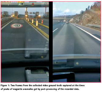
The tests were performed with the vehicle axes aligned MEMS-based Attitude and Heading Reference System MTi-G from Xsens (AHRS) on one side and the cheap three-axis magnetic sensor found in many smart phone devices on the other. For the latter an HTC One X was used with the Androsensor application used for the capture and logging. An additional smart phone recorded a video file which served as a ground truth source.
Data Analysis
In the first set of the experiments, the focus of the data analysis was focused on the isolation and identification of any eventual magnetic anomaly. However, due to the weak declination of the magnetic field attributed to the presence of the large ferromagnetic objects, the signal was obfuscated in a high (with respect to the signal) noise environment. This made the anomalies identification quite a challenge. The aim of the analysis was to perform a standard procedure on acquired date in order to build a geographical database of ferromagnetic objects.
Since both the sensors used measure the magnetic field in all the three dimensions, the first step was to calculate the magnitude of the magnetic field. Next a filter was applied in order to reduce the noise. The collected points were smoothed by calculating an average over a window of fixed width (S). This way a running average was achieved.
The smoothed data was subtracted with the time average of width W (local mean). Then the standard deviation was calculated in the same window. The deviations were then averaged once again over Q samples. This was defined to be the local mean deviation. A peak acquisition was triggered if the deviation was greater than the local mean deviation [6].
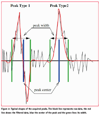
The last decision was to define the shape, amplitude, center and the width of the peak. As can be seen in the figure 2, the shape of the peaks was mainly of the two types. The amplitude and the width were not taken into account for the moment. The center was used to set the position coordinates of the anomalies. The center was set on zero crossing for the peak of the type 1 and its maximum for the type 2.
When the peaks were close to one another, so that it was meaningful to attribute them to the same source, they were merged into single event.
Results
This section provides a summary of the results obtained after the previously explained analysis for the different anomaly causing objects considered.
Crossing the railway power lines
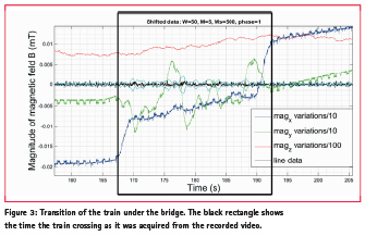
The effect of the passage of the train under a bridge near Črnotiče was measured. The results were expected to be interesting particularly due to the fact that the Slovenian railways use DC power lines to feed the trains’ electric motors. The DC current running through these lines should thus provide a static and almost constant magnetic field in the direction perpendicular to the lines. The question was whether this contribution to the magnetic field could be measured.
As it can be seen in the figure 3 the effect of the train passing under is of order of magnitude of 0.1 mT. Using the Ampere’s law an estimate of the electrical current needed to produce such a magnetic field can be calculated:
![]()
This gives the current in the order of magnitude of few kA which is perfectly sensible for a locomotive of 6MW fed with a 3kV power line. Furthermore, according to the recorded video the change of the magnitude completely coincides with the train passage. It should be noted that due to the high inclination of the railway in question the train compositions have at least two locomotives, one on the front and one at the tail. This leads to a conclusion that the change in the magnetic field should necessary be the consequence of the electrical current feeding the trains’ motors.
The small trend of almost linear increasing of the magnetic field could be attributed to the change of the terrain slope and the train needs to draw more current. At the same time no sensible explanation was found for the variations in the perpendicular directions. An early proposition was to attribute the variation to a possible magnetic properties of the transported ore. However, this would make a contribution in a random direction that would be isotropically distributed along the train composition. There are also some small variations on the order of magnitude of 1s in both directions that neither could be explained well.
Energy distribution lines
A similar effect was observed when driving under power distribution lines in the vicinity of Hruševje. The difference from the railway power lines is that the electrical power distribution in Slovenia has a frequency of 50~Hz. This is just on the Nyquist limit of our sampling rate (100~Hz).
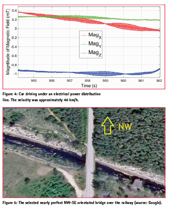
In the figure 4 an oscillation of the magnetic field can be observed that has an amplitude on the order of magnitude of ~0.1mT and frequency 50~Hz. Using the same reasoning as above, those effects can be easily contributed to the AC currents in the power line of the order of magnitude of few kA.
From the velocity sensors it can be seen that the car was driving at approximately 40 km/h. The variations of the envelope of the oscillations can be attributed to the high curvature at the location of transition or could be attributed to the under-sampling rather than the effect of different sources (each from a wire of a different phase); the latter would imply that the wires should be at least 20 m apart. A repeated experiment is needed by either increasing the sampling rate or driving at a slower velocity.
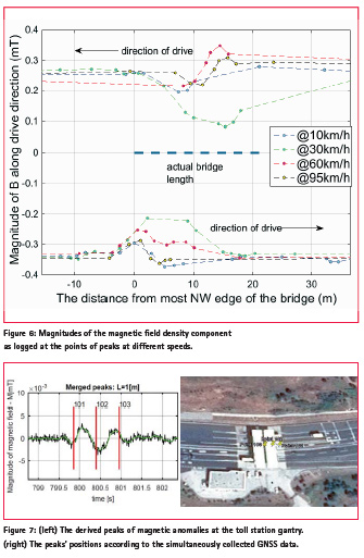
The bridge: Observed along drive magnetic magnitudes at peaks
The filtering algorithm was tested in the specific magnetic environment of bridge over railway, as shows the figure 5. Several tests at different speeds were performed to justify the admissible parameter set. When passing the bridge from each direction a significant behavior of transients i.e. the shapes and mean levels occurs at different speeds, as shows the figure 6. A very well magnetically defined most NW edge occurs, regardless of the speed.
Data collection on the roads
Inertial and magnetic field data were collected on the roads in the Littoral Region of Slovenia. The set of selected 400km of roads brings a set of different types of roads (local, regional and highway). Interestingly, very rare portal pillars were signed with magnetic signature, while most bridge structures and fences left at least their edges fingerprints.
As an example of still typical infrastructure object on Slovenian highways, a toll gantry is presented. A graph on the figure 7 shows regular fingerprint as get at the speed of 20km/h.
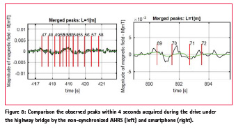
AHRS vs. smartphones data collection
In order to floor the crowdsourcing, a comparison of the AHRS and the smart phones built-in sensors was involved. For this purpose the measurements of the influence a highway bridge structure was used. As one can see comparing the figures 8 and 9, for its higher sampling rate (100Hz vs. 10Hz) the acquisition from AHRS unveils more details of the bridge, while the shape of the transient is quite similar and it also marks both edges of the bridge. The coordinates of the peaks as referenced by the smart phone shows the lower accuracy of its GNSS receiver.
We should emphasize that the repetition of the measurement gave similar results, regardless of the driving direction. This seems very promising and could potentially lead to a map of magnetic anomalies. A consideration on how to adapt the sensor to a vehicle is well investigated [5]. However, the demands for a person who takes part in crowd-sourcing to appropriately record the magnetic deviation curve of the vehicle before starting the data collection – is not very reliable. The significance of the uncalibrated data is poor for mapping [5], even in the case that they are well georeferenced and the influence of the local geomagnetic field is known for example from the INTERMAGNET exchange.

Conclusions
Along the road mapping and creating the world model automatically [3], [5] still remains a challenge, but according to the data processed so far, a good correlation between the peaks and presence of ferromagnetic structures obviously exists.
Since the non-investigated magnetic coupling of the car body and any drivenby ferromagnetic objects also influences the behavior, for any large acquisition attempt an automatic calibration approach has to be proposed. A potential contributor to the database should collect the georeferenced magnetic field data with at least 10Hz sampling frequency.
After establishing the confirmed physical distances between the peaks by appropriate processing, a certain Braille’s script of the road is expected. And only a skilled ‘finger’ is needed to read it.
Acknowledgements
COST action TU1302 Satellite Positioning Performance Assessment for Road Transport (SaPPART) is gratefully acknowledged for the motivation on strengthening the navigation solutions.
References
[1] F. Dionori et al., “State of the Art of Electronic Road Tolling”, project report MOVE/D3/2014-259, 2015, p.32.
[2] T.SloveniaTimes, “Motorway pileup death toll rising”, Jan. 2016.
[3] J. F. Raquet, “What’s Next for Practical Ubiquitous Navigation? World Models and Magnetic Field Maps”, Inside GNSS, Sep./Oct. 2013, pp.61-69.
[4] P.D. Groves, ”Principles of GNSS, Inertial, and Multisensor Integrated Navigation Systems”, Artech House, 2013.
[5] J. A. Shockley, “Ground Vehicle Navigation Using Magnetic Field Variation”, PhD thesis, 2012, pp. 1-186.
[6] F. Dimc, M. Bažec and A. Grm, “Extraction of magnetic field anomalies from objects in a road infrastructure” European Navigation Conference, Helsinki, Finland, Jun, 2016. pp. 1-7.


 (1 votes, average: 4.00 out of 5)


Leave your response!