| GIS | |
Detecting Changes in Coastline in United States and Malaysia
This paper highlights the accuracy of remote sensing/GIS in measuring/detecting morphological changes in the coastline |
 |
|
 |
|
 |
|
Emergent coastal structures such as groins, detached offshore breakwaters, and sea walls have been successfully adopted as coastal protection measures for many decades (Dean and Dalrymple, 2001: Silvester and Hsu, 1997). These type of structures are common in the US and Europe (Dean and Dalrymple, 2001), and even more so in Japan, where Seiji et al. (1987) reported the completion of over 4,000 emergent breakwaters by the mid-1980s. However, these types of highly intrusive and aesthetically unappealing engineering structures are becoming increasingly unpopular among the more environmentally aware modern communities. As a result, submerged breakwaters (SBWs), that do not impair amenity or aesthetics are becoming a preferred option for coastal protection (Burcharth et al., 2007: Ranasinghe and Turner, 2006; Lamberti et al, 2005;). Nonetheless, SBWs have rarely been adopted for coastal protection in the past and therefore, their efficacy remains largely unknown. Furthermore enhanced shoreline erosion has been reported in the lee of the structures at several SBW projects worldwide. Ranasinghe and Turner, (2006) carried out a comprehensive review on documented projects of submerged breakwater in different parts of the world. Unfortunately, not many of these types of projects are available. From the ten (10) projects reviewed, erosion was noticed at the lee of seven (7) of these projects. Studying this type of projects has become imperative. The mode and magnitude of salient formation behind these structures need to be well documented and analyzed. But unfortunately performing an actual beach survey for all these SBW projects in different parts of the world will be quite expensive considering the inter-continental nature of their location. Feasibly, the remote sensing and GIS technique would be an appropriate substitute. The role of remote sensing and GIS to study shoreline changes is invaluable through complementing the field surveys, which are difficult and expensive to carry out in shorter periods. Remote sensing has made it possible for easy access to valuable data remotely. Valuable data such as Light Detection and Ranging (LIDAR) and satellite images of all places in the world could be acquired remotely. Landsat TM and ETM+ data for most places around the globe are currently freely available for download from the US Geological Survey’s Earth Resource Observation and Science Centre (EROS). Over 29 years of Landsat TM and ETM+ data are available at no or low cost from EROS. A majority of this data is terrain corrected to the L1T level. This processing level has been shown to have a nominal horizontal accuracy of +/- 1 pixel or 30 m.
Objectives
The accuracy of such an advanced technique to measure/detect the morphology of coastline has been questioned by a lot of researchers, stakeholders and consultants in the field of coastal engineering. This part of a larger study will endeavor to detect the morphology of two coastlines in the US and Malaysia using the advanced technique of remote sensing/GIS, and emphasis will be placed on the accuracy of such a technique. The accuracy of such technique was determined by the following;
• Acquire remote sensing data in the form of LIDAR and medium resolution satellite images for places in the US and Malaysia respectively.
• Process and analyze the acquired data using remote sensing/GIS technique.
• Validate the medium resolution satellite images for Malaysia with actual beach profile survey.
Literature
Study Area
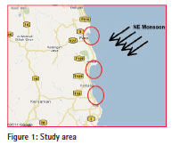
To validate the remote sensing data acquired for Kerteh, Malaysia a study area was chosen in Malaysia. The study area is located within a town called Kerteh in the district of Kemaman in Southern Terengganu, Malaysia, about 30 km or 20 minutes’ drive north of Chukai. Kerteh is the base of operations for PETRONAS in Terengganu, overseeing the oil platform operations off the state’s coast. Kemaman is a district of 2,536 km2 area with a population of 174,876. It’s geographical location is 4º 31′ 38″ N and 103º 28′ 9″ E. The stretch of the beach protected is approximately 2,100 m. The study area is characterized with much of its coast to be a series of large and small hook-shaped bays, fully exposed to direct wave attack (especially during NEmonsoon) from the South China Sea. The geomorphologic feature of Kerteh bay is such that its development is controlled by protruding headlands. Most of the bays along this region are considered to be in dynamic equilibrium. This is when constant supply of material from up-coast or within its embayment is passing through the bay and beyond the down-coast headland. The littoral drift rate, associated with the dynamically stable configuration of Kerteh Bay has been computed to be some 210,000 m3/yr of which more than 80% is transported during the NE-monsoon period
The cause of the coastal erosion at the study area Kerteh Bay was studied by Tilman et al (1993). Some major causes were highlighted by the researchers. The beach platform at Kerteh Bay is a continual long-shore sediment transport from upcoast to down-coast. Disruption of this dynamic stability may easily occur when up-coast sediment supply is (partly) cut off which can result into erosion of the coast leading to a larger indentation of the bay configuration. If the entire up-coast sediment supply is cut off, the bay would become even more indented until littoral drift ceases. Another factor identified is the cross-shore sediment transport, although it was reported that this factor doesn’t have as much effect as the long-shore sediment transport. The direction and intensity of this transport phenomenon are ruled by the wave steepness, geometry of the seabed slope and the size of the seabed particles. The beach will accrete at moderate wave conditions and recede under severe wave attack.
The third factor is the supply of sand by S. Kerteh River discharge. Unlike the larger rivers in the region such as S. Terengganu, S. Dungun and S. Kemaman, it was found that S. Kerteh River only drains a very limited catchment and it is unlikely that its sediment yield will be of significance for beach stability. The last factor identified as affecting the stability of the coastal area within Kerteh Bay is considered to be human activity, such as removal of natural dune systems and vegetation.
An interesting phenomenon that affects the coastal erosion at Kerteh Bay is the up-coast sediment supply from Paka Bay which is largely transferred into Kerteh Bay through offshore bar, bypassing at the northern end of the bay. The ‘supply point‘ on to the coast of Kerteh Bay is located immediately up-drift from Rantau PETRONAS Complex, which makes this coastal stretch particularly vulnerable to any disruption of the equilibrium situation. This is refl ected in the shoreline mapping from 1966 to 1987. The observed erosion over this period would indicate an average deficit in the up-coast sediment supply of some 40,000 m3/yr. The causes and persistency of this deficit in unknown, but quite likely originate from S. Kerteh infl uence (disruptive of bar bypassing) and from shore developments within the up-coast Paka Bay, undertaken since the late sixties.
From the findings of the cause of coastal erosion at Kerteh Bay, Tilmans and others proposed some mitigation measures. By careful examination of the geomorphologic situation of the Kerteh Bay and acknowledging the cause of erosion at the Rantau PETRONAS Complex, various defense schemes were proposed. An artificial supply of sand (beach nourishment, perched beaches), structures to prevent waves from reaching erodible materials such as bulkheads, seawalls, revetments and offshore breakwaters, and the last being structures to slow down the rate of littoral transport such as groynes (trapping the sediment) or offshore breakwaters (reducing the wave energy in the coastal zone) were all among the methods proposed.
The beach nourishment and use of three offshore submerged breakwaters were adopted for the purpose of mitigating the coastal erosion at the affected area as of the time of the study carried out by Tilmans et al (1993). Subsequently, after sometime erosion occurred at further north and south of the protected area. No doubt the findings of Tilmans and others have been of tremendous use for the mitigation of the coastal problem at a time. Their findings led to the construction of three submerged breakwaters with beach nourishment to mitigate the coastal problem at a specific time. The solution could be considered relatively effective considering the problem at that time, but no monitory survey has been carried out since the installation to evaluate the performance of these structures, but erosion has been noticed at the south and north of the protected area.
Remote sensing/GIS
Traditionally, morphological response of shoreline to structures is observed with the use of beach profile survey and other methods that involves physical measurement of changes at the site over time. Remote sensing can provide an alternative to this tedious, laborious and expensive exercise. Previous studies of monitoring topography and morph-dynamics of coastal flats using remote sensing imagery have focused on ‘waterline’ extraction. The waterline is defined as the instantaneous land-water boundary at the time of the imaging, while coastline or shoreline is the water at the highest possible water level (Niedemeier et al., 2005). The sea may be treated as an altimeter in this method, and the sea level may be determined by the data on tide height collected from original tide gauge records or obtained from hydrodynamic models.
Waterlines at different tide stages of a particular location can be corrected to obtain a particular datum-based shoreline using tidal correction models. Over the past decades, many studies have used satellite-derived data to ‘sketch’ waterlines at coastal areas and water bodies using both active and passive sensors, including synthetic aperture radar (SAR), near infra-red, shortwave infrared and thermal infrared images (Yamano et al., 2006). Among these satellite-based sensors, SAR shows prominent advantages in the waterline technique (Mason and Davenport, 1996), which can provide ground information regardless of cloud presence. Archived SAR data are, however, less available than commercial optical sensors (such as Landsat TM/ETM, Terra ASTER, SPOT, and IKONOS/Quickbird). Obviously, SAR sensor seems unlikely to be widely applied to coastal areas at present. In the passive optical sensors, higher spatial resolution is another attractive option because of their higher accuracy in waterline detection, but purchasing such images means higher costs (Yamano et al., 2006). For this practical reason, a cost/ benefit analysis of five satellite sensor bands (IKNOS band 4, Terra ASTER bands 3 and 4, and Landsat ETM+ bands 4 and 5) has been made by Yamano et al. (2006), and their work declares that Terra ASTER band 3 is the most cost-effective sensor for extracting waterlines with reasonable accuracy.
However, it should be noted that Terra ASTER is mainly observed on user demand and lacks routinely archived data. In this sense, it is impossible to obtain enough Terra ASTER data archives with various tide conditions in coastal areas for all the study areas of this research. The Landsat platforms have been providing scientists with mediumresolution satellite imagery for over 30 years. In 1970s, Landsat launched land mapping with a series of MSS satellites. In the early 1980s, the second generation of Landsat satellite TM added two more infrared bands and a thermal long-wave infrared band, and doubled the resolution capabilities of the multispectral bands. Later, Landsat 7 successfully introduced the Enhanced Thematic Mapper platform in 1999 and added a higher-resolution panchromatic band (15 m). TM became a popular platform providing repetitive synoptic, global coverage of multispectral imagery with relatively high-frequency, especially providing the preferred data source for the analysis of historical data sets.
Several researches have been carried out using Landsat Imageries for various purposes. Ryu et al., (2004) applied Landsat ETM+ satellite images to the study on the relationship between spectral refl ectance and the sedimentary environments on Gomso Bay, Korea. They concluded that remnant surface water in a tidal fl at is an important factor in influencing spectral refl ectance, and is affected by regional topography, grain size and the distribution of tidal channels. Zhao et al (2009) used Landsat imageries of Yangtze Delta, China to detect changes that have occurred over time. They obtained imageries for the period between 1987 and 2004, extracted the waterlines and used their corresponding tidal heights obtained from hydrodynamic models to construct a Digital Elevation Model.
Daniels Richard (2001) showed that an accurate shoreline/waterline extraction could be achieved using Landsat archived imageries when a tasseled cap transformation is used to convert the originals bands into new sets of bands with defined interpretations that are useful for vegetation mapping. The transformation is calculated by the taking the original images bands and creating a new set of output bands based on the sum of image band 1 times a constant plus image band 2 times a constant. The derived brightness, greenness, wetness Tasseled Cap bands will then be used as an input into ESRI unsupervised ISO classification algorithm to derive ten land use classes, and these 10 classes will be merged to obtain a binary classification (i.e., land and sea). He reported that the Tasseled Cap did a good job of differentiating between waves and beach, especially when the classifier option to leave 0.5% of the pixels was unclassified. The Tasseled Cap was unable to differentiate between land and sea for imageries with stratus clouds but this was solved by the use of NDVI band.
Materials & data
LIDAR
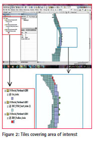
LIDAR data were acquired for the area of Palm Beach, United states in LAS format and converted to ASCII. Triangulated Irregular Networks (TIN) was generated from the xyz data contained in the ASCII format using the ArcGIS 10.1. The data were acquired based on tile scheme as shown in Figure 2 below. Data sets are chosen based on the tile that covers the respective study area of interest. As shown in Figure 2, four tiles were chosen for the data acquisition. These four tiles (with the green dots) covers the area of interest for this study.
Landsat 5 Satellite Images
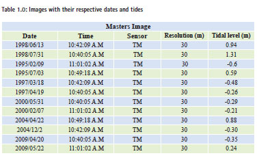
Landsat imageries from Landsat 5 were acquired for the Malaysia study area; imageries of 30 m spatial resolution were acquired from the Landsat platform. Landsat is known to be a platform that provides repetitive synoptic, global coverage of multispectral imagery with relatively high-frequency, especially providing the preferred data source for the analysis of historical data sets. Table 1.0 below shows the relevant information on the images acquired such as the date of images; time of image captured; the sensor that captured the images; resolution of the images and corresponding tidal heights of the images. The tidal heights were acquired using the hydrodynamic model.
Beach Profile survey data
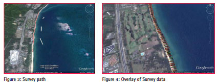
Beach profile survey is still the most accurate means of detecting changes in shoreline over time and was used for the validation of the remote sensing/GIS technique results. The Real Time kinematics survey method was adopted for this study. Real Time Kinematic (RTK) is a technique used to enhance the precision of position data derived from satellite-based positioning systems being usable in conjunction with GPS. It uses measurements of the phase of signal’s carrier wave rather than the information content of the signal, and relies on a single reference station to provide real-time corrections, providing up to centimeter-level accuracy. It has applications in land survey and in hydrographic survey. The survey path in which the survey was carried out is shown in Figure 3. The shoreline surveyed is about 3 km. Figure 4 shows the actual survey being overlaid in a Google earth image of the area surveyed.
Methodology
Processing of LIDAR data
The method of data acquisition for the LiDAR data for the Florida area in the US. These numerous ASCII format data were uploaded into ArcGIS interface as shown in Figure 5 and then converted to TIN as shown in Figure 7. Figure 6 below shows the work fl ow chart for this process.
TIN was generated for the ASCII data for 1999, 2004 and 2007 for the same area. This provided topographic information for these years for Florida, US. With the aid of a profile measuring tool in ArcGIS 10.1, the profiles at different sections covering the interested coastline were measured and compared for these years.
Processing of Landsat Images
The accuracy of shoreline extraction using remote sensing/GIS relies mostly on classification and tidal correction. Land cover classification has been the pivot that determines the accuracy of shoreline extraction, especially for medium to coarse spatial resolution imageries. Previous studies have suggested that the calculation of a single transformation, the Normalized Difference Vegetation Index (NDVI) or the use of the Infrared Band (NIR) may be suitable for water delineation and the values of the band ’sliced’ to identify water, bare soil, and vegetated lands. However, a majority of these studies dealt with calm water environment unlike what’s applicable to the study area of this research. The study area is characterized with white capping along the shoreline.
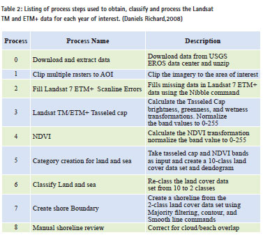
This study is based on Daniels Richards (2008), process (Table 2) of extracting shoreline from Landsat TM and ETM+. He used this method to derive ocean shorelines for 1989, 1995, 1999, 2010, 2011 and 2012 for Southwest Washington and Northwest Oregon. The shoreline changes were analyzed for a 102 km-long coastline. The changes rates from 1995 to 1999 were compared to published rates obtained from orthophotography and an R-squared of 0.79 was obtained. This method was further improved by correcting the extracted shoreline tidally. Two tide corrections models were used and the equiangular triangle tide model was selected based on its closeness in slope value to the slope value of an actual survey.
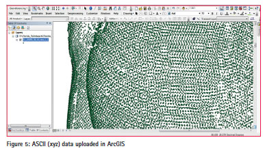
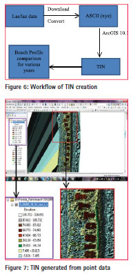
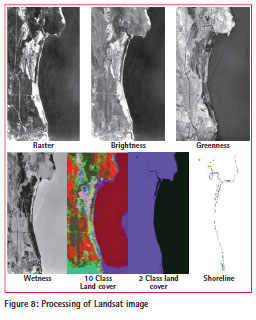
Figure 8 shows a processed image from the raster form to the extracted shoreline. As highlighted in table 2 above, after the successful download of the Raster image, it’s then clipped (subset). Landsat 5 has 7 bands and 6 of these bands were transformed. Bands 1-5 and band 7 are merged using the Tasseled Cap, which will give an output of Greenness, Brightness and Wetness transformation. Bands 4 and 5 are then separately combined to give an output of NDVI. These outputs – greenness, brightness, wetness and NDVI are used as an input to create a 10 class land cover data set and dendogram. The 10 class land cover data set is then re-classified to obtain a 2 class land cover. A distinctive line (shoreline) is obtained from the 2 class land cover by the means of vectorization.
Estimation of tidal level
Hydrodynamic model was used for the purpose of estimating the tidal level for this study. Even though some tide gauges were available at some distances away from the study area, they could not be used because a tidal level difference of about 1 meter was observed between the tide gauges. Therefore, a hydrodynamic tidal model was used to determine the height of the sea surface at various times of image capture.
Shoreline determination
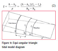
To accurately determine the actual shoreline for each year, the equi-angular tidal correction method (Figure 9) was used. Shoreline is considered to be the interface between land and sea. Instantaneous waterline at the time the various images were captured cannot be regarded as the shoreline. This instantaneous waterline is the shoreline position based on the tide at the time the image was captured. If a low tide for the same image is compared to a high tide of same image on the same day, it will definitely show that erosion has occurred over this very short span time – which is a misconception.
The equi-angular triangle model involves the extraction of two waterlines l1l1 and l2l2. The waterlines were extracted using the method described in the section above. The sea surface was regarded as an altimeter, the altitude of which was determined using the hydrodynamic model referred to also in the section above. The respective waterlines heights h1h1 and h2h2 were assigned using the tidal harmonic model. Thus, the bottom slope, ρ, was defined by Equation (1);
![]()
The Mean Higher High Water of 1995-96 was used as the tidal datum (hh) which was obtained from the tidal level standard port. It was assumed that the beach moves offshore or onshore with the same bottom profile (Huang et al., 1994). Thus, the waterlines were shifted to the tidal datumbased shoreline position based on the equi-angular theory as shown in Figure 9. The shifted distance, l, was estimated as;
Processing of Actual beach survey data
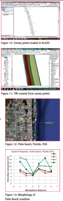
Survey exercise was carried out at the study area of Kerteh, Malaysia, in October 2012. The data were acquired using the Real Time Kinematic (RTK) method. The survey data were extracted from the RTK equipment in the ASCII format (xyz). These data were uploaded in the ArcGIS interface as shown in Figure 10. These point data were then converted to TIN as shown in Figure 11.
Results and discussion
Palm Beach, Florida, USA
Profiles of cross-sections created from TINs for the years 1999, 2004 and 2006 were compared to deduce the changes that must have occurred in the coastline of Palm Beach. Figure 12 shows the section of the beach in which the profile was measured. It was observed that most of the profiles analyzed showed almost similar morphology on the coastline. Henceforth, just one of the profiles will be discussed in this paper.
The cross-section of the profile that is situated in the middle of the coastline is selected for discussion in this paper. The changes that occurred at the Palm Beach coastline from 1999 through 2004 and 2007 are as shown in Figure 13. From the graphical representation it can be deduced that between 1999 and 2004, there was erosion. But also from the same graph (Figure 13) it can be deduced that between 2004 and 2007 there was accretion.
Kerteh Bay, Malaysia
Change analysis of the processed and corrected shoreline from the satellite images as described in section 5, were carried out with the Digital Shoreline Analysis System (DSAS). The DSAS plug-in computes rate-ofchange statistics for a time series of shoreline vector data. It works within the Environmental Systems Research Institute (ESRI) Geographic Information System (ArcGIS) software. Amongst the statistics computation, this plugin computes are Net shore Movement (NSM; Shoreline Change Envelope (SCE); End point rate (EPR); Linear regression rate (LRR); Standard Error of Linear Regression (LSE); Confidence Interval of Linear regression (LCI); R-squared of Linear Regression (LR2); Weighted Linear Regression rate (WLR); Standard Error of Weighted Linear regression (WSE); Confidence interval of weighted Linear regression (WCI); R-squared of linear regression (WR2) and Least median of squares (LMS).
To better understand the morphdynamic process that has occurred at the study area over the period of 1988-2009, the study area is broken in parts as shown in Figure 14.
The Staff Quarters is situated in the northern part of the coastline studied, while the golf course and school are situated in the middle and southern parts of the coastline respectively. Figure 15 through Figure 17 shows the graphical representation of the morphology over time.
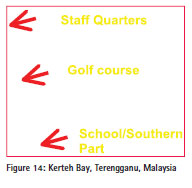
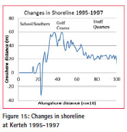
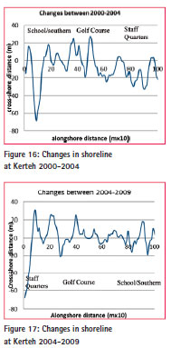
Figure 17 shows a graphical representation of the morphological process as obtained from the analysis of satellite images of the Kerteh. The analysis contained in this figure is based on the process that occurred between 1995 and1997. It shows accretion occurring at most parts of the coastline in this year slice. The magnitude of accretion at the beach directly in front of staff quarters can be approximated to be 35-40 m of width. This means the beach in front of the staff quarters widens up to about 35-40 m. The beach in front of the golf course also widened up for the same year slice but not as much as the beach in front of the staff quarters. The width of the beach in front of the golf course increases in width by a value of 20-25 m and for the same year period the school had its beach increased by a smaller value of 18-22 m.
For the year slice of 2000-2004, erosion rather than accretion was observed at the study area remotely. Erosion of magnitude of 18-20 m was observed in front of the staff quarters. This is well depicted in Figure 16 as shown above. The magnitude of erosion for the beach in front of the golf course is between 5-22 m, not as much erosion as compared to the magnitude of erosion in front of the staff quarters. Erosion in front of the school for this period was put at 15-27 m of average magnitude.
Unlike the morphological process observed for the year slice 1995-1997 and year slice 2000-2004, both erosion and accretion were noticed at the study area from the images processed for years between 2004-2009. While accretion was observed to have occurred at the beach in front of staff quarters and school, erosion was observed at the golf course for the same year slice. The staff quarters and the school have accretion magnitude of 5-10 m and 5 m respectively, and the golf course had erosion value of 5 m as shown in Figure 17 below.
Validation
Validation was done based on comparison of slopes obtained from the processed images as described in section 5, with slopes obtained from actual field study for the same period of images processed. The date of the field study used for the validation was sometime in October 2012 and this was compared to slopes of images of the same period (2012) and place. Digital Terrain Model (DTM) was created from the survey data (Figure 10) generated from this field survey using the triangulation method of interpolation as show in Figure 11 above.
Conclusion
Measuring/detecting shoreline changes remotely would one day be carried out solely from remote places of the offices of stakeholders. The accuracy of such an advanced technique can only get better with more research.
The use of LIDAR has achieved some level of accuracy as compared to the medium resolution images of 30 m spatial resolution.
Conclusively the accuracy of the LIDAR data could be put at 0.6 m vertical accuracy which makes a valuable data for remote sensing. Past research have also reported the accuracy of using Landsat 5 images and the accuracy is mostly put at ±30 m, but with the method described in this paper it is believed the accuracy has been tremendously improved.
The accuracy of the Landsat 5 images analyzed in this study can be correlated to the difference in slope of the measured beach slope and the calculated beach slope. Beach Slopes measured on the site for year of 2012 for the intertidal zone in front of the golf course is 0.63-0.70 and the slope obtained remotely from the images of the same place are put at 0.107.
References
Dean R. G and R. A Dalrymple, Coastal Processes with Engineering Applications, Cambridge University Press (2001) 488p.
Lamberti, A., Mancinelli, A. Italian experience on submerged barriers as beach defence structures. Proc. 25th International Conference on Coastal Engineering. ASCE, Orlando, USA, pp. 2352-2365.
Mason, D., Hill, D., Davenport, I., Flather, R., Robinson, G., (1997). Improving inter-tidal digital elevation models constructed by the waterline technique. In: Third ERS Symposium, Florence, Italy, pp. 1079-1082.
Niedermeir, A., Hoja. D., Lehner, S., (2005). Topography and morphodynamics in the German bright using SAR and optical remote sensing data. Ocean dynamics 55, pp. 100-109.
Pope, J., & Dean, J. L. (1986). Development of design criteria for segmented breakwaters, Proceedings 20th international conference on coastal engineering. American Society of Civil engineers, Tapei. Pp. 2144-2158.
Ranasinghe R., Hacking N., and Evans P., Multi-function artificial surf breaks: a review, Report No. CNR 2001.015, NSW Dept. of Land and Water Conservation, Parramatta, Australia (2001)
Ranasinghe R., Turner I., and Symonds G., Shoreline Response to Submerged Structures: A review Coastal Engineering (2006). Vol. 53, 65-79
Ranasinghe R. and S. Sato, Beach morphology behind impermeable submerged breakwater under obliquely incident waves. Coastal Engineering (2007). Pp. 1-24
Richard C. Daniels (2008). Using ArcMap to Extract Shorelines from Landsat TM & ETM+ Data. Thirty-second ESRI International Users Conference Proceedings, San Diego, CA.
Ryu, J.H., Kim, C.H., Lee, Y.K., Chun, S.S., Lee, S., (2004). Detecting the intertidal morphologic change using satellite data. Estuarine, Coastal and Shelf Science 78, 623-632.
Seiji, W. N., Uda, T., Tanaka, S., Statistical study on the effect and stability of detached breakwaters. Coastal Engineering in Japan 30 (1), 121-131.
Silvester R. and Hsu J., Coastal stabilization, World Scientific Publishing Co., Singapore (1997) 578 pp.
Stauble, D. K., Tabar, J.R., Smith, J.B., (2000) Performance of a Submerged breakwater along a hardbottom influenced coast: Vero Beach, Florida. Proc. 13th National Conference on Beach Preservation Technology, Melbourne, Florida, USA, pp. 175-190.
Tilmans W.M.K, W.H.G. Klomp & H.H. de Vroeg 1992. Coastal erosion – the Kerteh Case. Analysis of causative factors and mitigative measures using dedicated mathematical modeling tools, International Colloquim on Computer Applications in Coastal and Offshore Engineering.
Yamano, H., Shimazaki, H.S., Matsunaga, T., Ishoda. A., McClennen, C., Yokoki, H., Fujita, K., Osawa, Y., Kayanne, H., (2006). Evaluation of various satellite sensors for waterline extraction in a coral reef environment: Majuro Atollm Marshall Islands. Geomorphology 82, 398-411.
Zhao, B., Guo, H., Yan, Y., Wang, Q., Li, B., (2008). A simple waterline approach for tidelands using multitemporal satellite images: a case study in Yangtze delta. Estuarine, Coastal and Shelf Science 77, 134-142.
The paper was presented at 9th National GIS Symposiun in Saudi Arabia at Damman during April 28-30, 2014.


 (5 votes, average: 4.00 out of 5)


Leave your response!