| Geodesy | |
PGM2016: A new Geoid Model for the Philippines
In 2016, the PGM2014 was re- computed into PGM2016 using the reprocessed and densified land gravity data (from 1261 to 2214 points) |
 |
|
 |
|
 |
|
In 2014, a preliminary geoid model has been computed for the Philippines i.e., Philippine Geoid Model 2014 (PGM2014), with the technical assistance of the National Space Institute, Technical University of Denmark (DTU-Space) using data from land gravity, airborne gravity, marine satellite altimetry and the newest satellite gravity data from the GOCE mission release 5. Digital terrain models used in the computation process was based on 15” SRTM data. The model is computed in a global vertical reference system then fitted to the ITRF GNSS/Leveling and validated with RMS value of 0.50m. In 2016, the PGM2014 was re- computed into PGM2016 using the reprocessed and densified land gravity data (from 1261 to 2214 points). Significant improvements can be seen in the reprocessed gravity data and GPS/Leveling (RMS = 0.040m). Further densification of the land gravity (in towns and cities) to 41,000 points will be conducted from 2017 until 2020 to refine the geoid. Re-computation will be done for the new version of the geoid as new gravity data comes in. GRAVSOFT system of FORTRAN routines developed by DTU-Space and Niels Bohr Institute, University of Copenhagen was used in computing the Philippine geoid.
Introduction
Vertical coordinates (i.e. Heights) of points are referred to a coordinate surface called Vertical Datum. The universal choice of a vertical datum is the geoid – the reference surface for orthometric and dynamic heights (Vanicek, 1991). It is an equipotential level surface of the oceans at equilibrium, proposed by C.F. Gauss as the “Mathematical figure of the earth” (Dr. Bernhard Hofmann-Wellenhof, 2005).
With the advent of Global Navigation Satellite Systems (GNSS), it has become much easier to estimate Mean Sea Level (MSL) elevations using a geoid model. Applying a geoid model in GNSS surveys will eliminate the conduct of levelling. A geoid model is a surface (N) which describes the theoretical height of the ocean and the zero-level surface on land. In a modern vertical reference system, the geoid is required to obtain orthometric height H (“height above sea level”) from GPS by
![]()
Where hGPS is the GPS ellipsoidal height, and H the levelled (orthometric) height. In the Philippines, determination of elevation H of points and Benchmarks (BMs) was normally conducted thru Geodetic Levelling, a tedious process that hinders the densification of BMs during the early times.
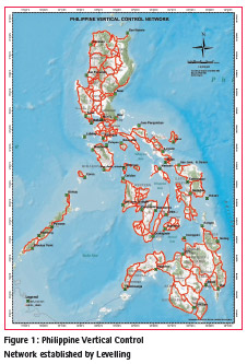
In 2007, during the Philippine Reference System 1992 (PRS92) Campaign, 22,851 BMs were established along major roads nationwide with a maximum divergence of between two level runs (1st Order Accuracy). These first order level networks were connected to their respective reference tidal BMs to provide local MSL elevation. Figure 1 shows the Network of Level Lines with their corresponding Tide Gauge Stations.
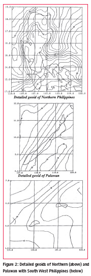
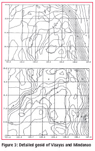
The first attempt of computing a preliminary gravimetric geoid for the Philippines is through the Natural Resources Management Development Project (NRMDP) in 1991. Land gravity data and altimetrically-derived anomalies at sea and OSU89A to degree and order 360 (reference global model) were used. Biases between the gravimetric N and GPS/ Levelling were found ranging from 2-6 m nationwide (Kearsley, 1991). Figures 2 and 3 shows the computed detailed geoids of the Philippines.
The making of Philippine Geoid Model 2016 (PGM2016)
In October 28, 2014 with the technical assistance of National Space Institute -Denmark Technical University (DTUSpace) and funding from National Geospatial-Intelligence Agency (NGA), a preliminary geoid model, Philippine Geoid Model 2014 (PGM2014) has been computed for the country using the data from land gravity, airborne gravity, marine satellite altimetry and the newest satellite gravity data from the GOCE mission release 5 with an accuracy of 0.30meters. In this paper, the computation of the PGM2014 will be discussed then its re-computation into PGM2016.
The airborne gravity survey
The success of the first long-range airborne gravity survey in Greenland 1991- 92 by the group of US Naval research Laboratory, in cooperation with NOAA, NIMA and Danish National Survey paved the way for the use of airborne gravity in filling the intermediate wavelength bands between satellite gravity, e.g. GRACE and GOCE (R. Forsberg & Olesen, 2010) for accurate geoid modelling. There is now full operational capability of collecting seamless airborne gravity data across land and marine areas at 1-2 mGal r.m.s. accuracy and at around 4-6 km resolution due to the new gravity acceleration sensors and improved GPS processing methods.
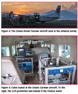
After their successful airborne gravity campaigns in the other regions of the world (e.g., Malaysia, Mongolia, Ethiopia, South Korea, Nepal), DTU-Space conducted the airborne gravity survey in the Philippines on March until May of 2014 using a Cessna Caravan aircraft. This is part of the project to improve the global gravity field model EGM2008 under the umbrella of the NGA – Danish Geodata Agency BECA agreement. Figures 4 and 5 shows the aircraft used in the Philippine airborne gravity survey and its cabin layout respectively.
The following instruments were used:
– LaCoste and Romberg Air/ Sea gravimeter S-38
– Chekan AM gravimeter #24
– Javad Lexon GPS receiver
– Javad Delta GPS receivers
– Novatel dual frequency aircraft GPS antenna
– Power rack with DC/AC inverters, UPS etc.
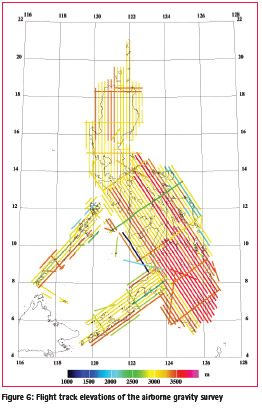
GPS reference stations operated in all airports together with active geodetic stations of NAMRIA were used as base stations in computing the position of the aircraft. AUSPOS online positioning provides the coordinates of the reference stations (in ITRF2008) with an estimated accuracy of 0.50 to 2cm in vertical. Aircraft trajectories were computed with waypoint software package from Novatel (Calgary, Canada) using precise ephemeris from International GNSS Service (http:// igscb.jpl.nasa. gov/). Parking spots were tied to NAMRIA first order gravity stations using Scintrex CG-5 gravimeter.
Mean altitude for all flights was 3185m with a terrain clearance of 545m above mountains and 3760m in lowlands. Figure 6 shows the colorcoded flight track elevations.
Free –air gravity anomalies at aircraft level are obtained from:
![]()
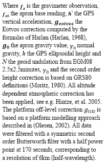
Apron base readings were performed each day after the flight and approximately every second day before the flight to monitor drift of the gravimeter and for proper connection of airborne readings to the gravity network.
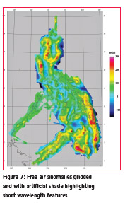
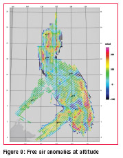
Figures 7 and 8 shows the gridded and acquired free air anomalies at flight altitude. Colour agreement at cross lines indicate consistent data. Closer examination of the misfit in the 289 line intersections shows a 3.7 mGal RMS error indicating 2.6 mGal average noise level.
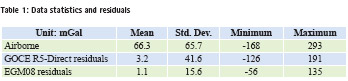
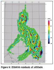
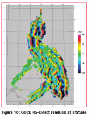
Comparison to EGM08 shows significant differences in many places amounting to more than 130mGal over SE Mindanao, see Table 1 and figures 9 and 10.
Gravimetric geoid computation – principles
The PGM2014 is computed by the GRAVSOFT system, a set of Fortran routines developed by DTU-Space and Niels Bohr Institute, University of Copenhagen (Forsberg R, 2008). It forms the base of major recent geoid computation projects, such as the joint Nordic “NKG” geoid models, undertaken as joint geoid model computations of the Nordic and Baltic countries (R. Forsberg, D. Solheim & J. Kaminskis, 1996) under the auspices of the Nordic Commission for Geodesy (NKG), as well as the OSGM02 geoid model of the UK and Ireland (R. Forsberg et al., 2002), and several national geoid models done from airborne surveys in recent years (Malaysia, Mongolia, Indonesia and others).
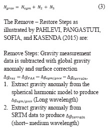
The “remove-restore” technique was used in computing the geoid, where a spherical harmonic earth geopotential model (EGM/GOCE combination) is used as a base. The geoid is divided into three parts namely: the global contribution , a local gravity derived component N2, and a terrain part N3.
The EGM08 model is incorporating GRACE satellite data, which determines the error spectrum of the EGM08 up to spherical harmonic degree 80 or so. New satellite data from the GOCE mission have recently been made available by the European Space Agency, for details see www.esa.int/goce. The latest GOCE spherical harmonic model (“Direct” Release 5 model), complete to degree and order 280 was used to update EGM08 field in the following way:
– EGM08 used unchanged in spherical harmonic orders 2-80, and from 200 up
– GOCE R5 direct model used in band 90-180
– A linear blending of the two models done in bands 80-90 and 180-200
The mixed spherical harmonic model (termed EGM08/GOCE) has been used to spherical harmonic degree N = 720, corresponding to a resolution of 15’ or approximately 28 km. From the recent DTU geoid projects in France (Auvergne), Malaysia, and Nepal, this resolution appears to be a good ”trade off” between the full resolution of EGM08 (degree 2160) and the local gravity data. Because the full-resolution gravity data used in the construction of EGM08 is classified, there is no good information on the quality of the errors in EGM08 at the high wavelengths in SE Asia, and only 15’ mean gravity data are assumed to be underlying EGM08. All spherical harmonic computations were done in a grid using the geocol17 program in grid mode.
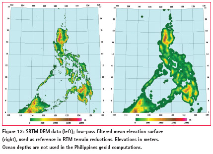
The terrain part of the computations were based on the RTM method, where topography is referred to a mean elevation level, and only residuals relative to this level is taken into account. The mean elevation surface were derived from the SRTM 15” detailed model through a moving average filter with a resolution of approximately 20’ (37 km; slightly longer than the 15’ data resolution implied by spherical harmonic degree 720, in order to have a more smooth residual gravity signal ). The difference in resolution between reference field and RTM is not a theoretical issue, as the remove-restore method takes any “double accounted” topography into account fully.
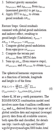
The method for the gravimetric geoid determination is spherical FFT with optimized kernels. This is a variant of the classical geoid integral (“Stokes integral”), in which there is a proper weighting of the long wavelengths from EGM08 and the shorter wavelengths from the local gravity data. Mathematically it involves evaluating convolution expressions of form
![]()
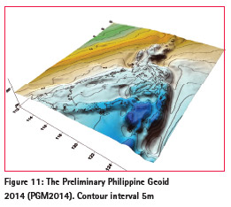
The geoid is computed on a grid of 0.025° x 0.025° resolution (corresponding to roughly 2.7 x 2.5 km grid). The area of computation is 04°-22°N and 112-128°E, covering the Kalayaan Islands of West Philippine Sea. Computations was based on least squares collocation and Fast Fourier Transformation methods which involve 1440 x 1280 grid points corresponding to 100% zero padding. The data are gridded and downward continued by least squares collocation using the planar logarithmic model. GRAVSOFT programs such as gpcol1, spfour, gcomb, geoip are involved in the process. Figure 1 1 shows the PGM 2014 at 5m contour .
The final gravimetric geoid solution was computed by the following steps:
– Subtraction of EGM08GOCE spatial reference field (in a 3-D “sandwich mode”)
– RTM terrain reduction of surface gravimetry, after editing for outliers
– RTM terrain reduction of airborne gravimetry
– Reduction of DTU-10 satellite altimetry in ocean areas away from airborne data
– Downward continuation to the terrain level and gridding of all data by least-squares collocation using a 1° x 1° moving-block scheme with 0.6° overlap borders
– Spherical Fourier Transformation from gravity to geoid – Restore of RTM and EGM08GOCE effects on the geoid
– Correction for the difference between quasigeoid and geoid (using a Bouguer anomaly grid)
– Shifting of the computed geoid by +80 cm to approximately fit to Manila tide gauge datum
Data used and Quality Control for the geoid computation
The PGM 2014 is based on the following data:
– Airborne gravity data
– Land gravity from NAMRIA, reformatted to GRAVSOFT and mildly edited
– DTU10 global gravity anomalies from multi-mission satellite altimetry (Selected only in the open ocean area, away from the airborne gravity)
– SRTM 15” DEM data for the region
– EGM08 and GOCE RL5 satellite data
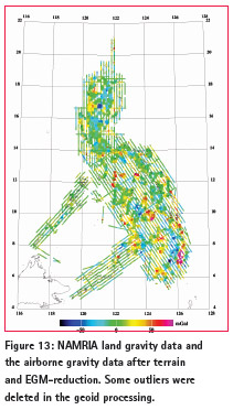
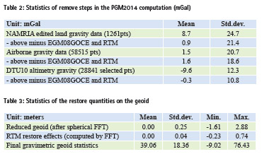
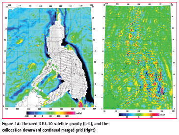
Some plots of the used and processed data are shown in the Figures 12-14. The available data from the airborne and surface sources were quality controlled through plotting of the EGM08/ GOCE and terrain reduction residuals, showing a few (< 1%) obvious surface gravity outliers, which were deleted in the final geoid processing. The overall EGM/GOCE and RTM terrain “reduce” statistics for the data are shown in Table 2. Overall this statistics is good, with relatively small bias and standard deviation for all data sets.
Geoid processing results
The plots in the sequel shows the intermediate results of the final removerestore geoid processing (“geoid.gri”), computed with full 3-dimensional modelling, going via the quasigeoid to the classical, final geoid.
The final geoid covers the region 4-22°N, 112-128°E, and has a resolution of 0.025° x 0.025°. The airborne and surface gravity data were gridded by spatial least squares collocation (gpcol1, using covariance parameters √C0 = 18 mgal, D = 6 km, T = 30 km). A priori errors assumed were 2 mGal for both the airborne data and the surface data (averaged in 0.025° blocks), and 5 mGal for DTU-10. The collocation downward continuation was done in 1° x 1° blocks, with 0.6° overlaps.
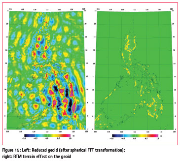
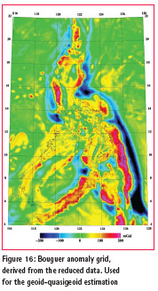
For the spherical FFT transformation of gravity to geoid, 3 reference bands were used. Figure 15-16 shows the primary data grids done in connection with the geoid processing. The final geoid “restore” statistics is shown in Table 3.
GPS/Levelling data comparison and fitted geoid
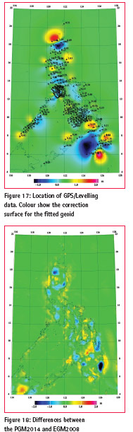
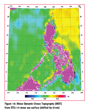
A set of 190 GPS data in ITRF2005 levelling benchmarks was used to compare with the final geoid. These GPS data showed large errors relative to the geoid, with large outliers in some regions, likely due to a combination of geodynamic effects, levelling and GPS errors. The rms fit is 0.5 m; it is therefore not possible to use these data for validation of the geoid. Figure 17 shows the offset values, and the geoid correction surface for a fitted geoid ph_geoid_fit (corrector surface gridded with 80 km correlation length, and GPSlevelling apriori error of 10 cm). Fig. 18 shows the PGM2014 comparison to EGM2008; large improvements are seen, especially in the south. Fig. 19 shows a comparison to the DTU10-MSS, i.e. the MDT, shifted by -91 cm to take into account the different reference systems.
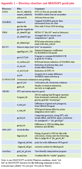
The PGM2014 files are given as GRAVSOFT grids, and can be interpolated by the GUI program grid_int (or the command line program “geoid”), provided to NAMRIA as part of the computations, along with the general software and geoid job setups (Appendix 1).
Re-computation of the geoid
To further improve a geoid model, Professor Forsberg in his paper “Towards a cm-geoid in Malaysia” (R. Forsberg, 2003) recommends the following:
– Levelling networks must be carefully analysed for adjustment errors
– Connections and antenna height errors of GPS data on benchmarks must also be revisited and re-analysed
– Erroneous points (geoid outliers) must be resurveyed by Levelling and GPS
– New GPS-fitted version of the geoid must be computed as new batches of GPS-Levelling data, additional gravity surveys in major cities and GPS users height problem reports comes in.
In 2015 NAMRIA started the recomputation of the PGM2014 with the help of Professor Forsberg. The densification of land gravity stations was conducted in some major cities of the country. Also, the GPS-levelling data was re-analysed, corrected and outliers deleted.
Land Gravity Data
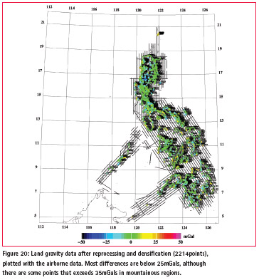
In this re-computation, the original airborne and satellite data processing results were used, only the densified land gravity data (2214 points to date) were reprocessed and quality controlled. Figure 20 shows the new plots of the land and airborne gravity data. Significant improvements can be seen in the land data (thicker dots). Most dots are in green, some yellows and light blue (i.e., 25-50 mGals difference in mountainous areas).
GPS/Levelling Data
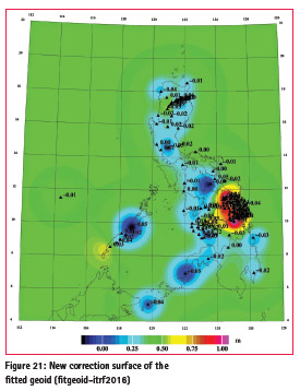
101 out of the 190 GPS/Levelling data on BMs remain (after cleaning up for outliers) and used as validation points. After fitting the new GPS/Levelling, the RMS now is 0.054m with a minimum and maximum offset value of -0.124m and 0.169m respectively. This improvement is mainly due to the removal of erroneous levelling points. More points will be added to the GPS/Levelling data as the re-adjustment of the levelling network progresses. Figure 21 shows the offset values and the new geoid correction surface for the ITRF-fitted PGM2016.
Philippine Geoid Model 2016
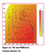
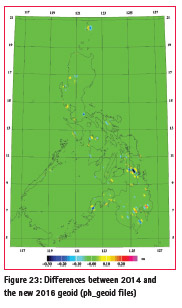
The PGM2014 was re-computed to the new PGM2016 using additional land gravity stations combined with the same airborne and satellite gravity data. More land gravity data (up to 41,000) will be added from 2017 until 2020 in order to re-compute a new version and further refine the Philippine geoid. Figure 22 shows the new PGM2016 and its plotted differences with PGM2014 in figure 23. There are differences in most parts of the country as big as 0.30m.
References
Dr. Bernhard Hofmann-Wellenhof, D. H. M. (2005). Physical Geodesy (pp. 46). Forsberg, R. (2003). Towards a cm-geoid for Malaysia. Paper presented at the geoid computation workshop in Kuala Lumpur.
Forsberg R, C. C. T. (2008). Overview manual for the GRAVSOFT Geodetic Gravity Field Modelling Programs (Technical Report, 2nd ed.): DTU-Space.
Forsberg, R., D. Solheim & J. Kaminskis. (1996). Geoid of the Nordic and Baltic area from gravimetry and satellite altimetry. Paper presented at the Symposium on Gravity, Geoid and Marine Geodesy, Tokyo, 1996. Forsberg, R., & Olesen, A. V. (2010). Airborne gravity field determination Sciences of Geodesy-I (pp. 83-104): Springer.
Forsberg, R., Strykowski, G., Iliffe, J., Ziebart, M., Cross, P., Tscherning, C. C., . . . Finch, O. (2002). OSGM02: A new geoid model of the British Isles. Gravity and geoid, 3.
Harlan, R. B. (1968). Eotvos corrections for airborne gravimetry. Journal of Geophysical Research, 73(14), 4675-4679.
http://igscb.jpl.nasa.gov/.
Kearsley, A. H. W. (1991). Evaluation of the geoid of the Philippines (Vol. 1): SAGRIC International. Moritz, H. (1980). Advanced physical geodesy. Advances in Planetary Geology, 1.
Olesen, A. V. (2002). Improved airborne scalar gravimetry for regional gravity field mapping and geoid determination. Faculty of Science, University of Copenhagen.
PAHLEVI, A., PANGASTUTI, D., SOFIA, N., & KASENDA, A. (2015). Determination of Gravimetric Geoid Model in Sulawesi–Indonesia. Paper presented at the FIG Working Week.
Vanicek, P. (1991). Vertical datum and NAVD88. Surveying and Land Information Systems, 51(2), 83-86.


 (No Ratings Yet)


Leave your response!