| GNSS | |
GNSS data for ionosphere characterization
The increasing number of GNSS receivers enables comprehensive studies of ionosphere. Different products derived from calculated ionization levels give insight in ionospheric conditions and dynamics |
 |
|
 |
|
Global Navigation Satellite Systems’ (GNSS) performance is affected by ionosphere. Sudden variations in ionization levels can increase the pseudorange errors and even cause loss of lock on some of the visible satellites, lowering the positioning accuracy and availability. Logically, GNSS can benefit of deeper understanding of ionospheric behavior and the processes behind it. On the other hand, GNSS and their wide spread receiver networks are nowadays the main source of data on ionosphere, alongside ionosondes, low Earth orbit (LEO) satellites and incoherent scatter radars. The increase in the number of GNSS multi-frequency receivers which provide publicly available data, usually in Receiver Independent Exchange Format (RINEX), deepens our knowledge of ionosphere, possibly enabling better correction of ionospheric errors in the future.
GNSS derived ionospheric data
The ionospheric conditions are affected by local time, geomagnetic coordinates, season, solar activity and geomagnetic activity. Together, these factors influence the structure and ionization levels in the ionosphere. Even though GNSS receivers do not provide data on ion composition in the ionosphere nor on the height of ionospheric layers and the associated electron density, they provide invaluable data which can characterize the ionospheric conditions. Signal phase and Signal-to-Noise Ratio (SNR) can be used to identify ionospheric scintillation, i.e. small plasma bubbles with density different than the surrounding plasma, which usually appear in polar and equatorial regions and can cause loss of lock on satellite signals. In order to provide indices on amplitude and phase scintillation, a 50 Hz or 100 Hz raw data output from GNSS receiver is required, but such receivers represent only a minority of all the deployed receivers, as the standard RINEX data rate is 30 s. On the other hand, Total Electron Content (TEC), which is proportional with the ionospheric signal delay, can be derived from any dual frequency receiver. The ionospheric error is usually quantified with TEC units (TECU), which equal 1016 electrons/m2. One TECU on GNSS L1 frequency (1575.42 MHz) contributes with 0.16 m pseudorange error.
TEC is calculated for every satellitereceiver pair. In order to geotag it, based on receiver and satellite locations, coordinates of a point on the path between the satellite and the receiver, situated on height of 350 km are calculated. The height of 350 km is the height where the electron density in the ionosphere is the highest. Vertical TEC (VTEC), derived from Slant TEC (STEC), is pinned to the calculated coordinates.
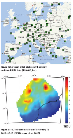
Most of the receivers support multiple GNSS constellations. A receiver situated in low and middle latitudes can usually receive signals from about 15 GPS and GLONASS satellites visible above the horizon, and slightly less towards the poles because of the constellation inclination in respect with the equatorial plane. With emerging BDS and Galileo systems, the number of visible satellites is even higher. Therefore, each GNSS receiver produces TEC data on 15 or more locations with different azimuths, and with distance up to 900 km from its location. Increasing the number of receivers increases the covered area and the density of points with calculated TEC, enabling interpolation and geographic representation of the collected data. Europe is a good example of a region well covered by GNSS stations with publicly available RINEX data, as can be seen in Figure 1.
VTEC values depict the current state of the ionosphere over a region of interest. In order to avoid appearance of faulty data, it is recommended to calibrate the values and to not to use data of satellites with low elevation, as such data are severely affected by multipath and mapping function errors. An example of the most commonly used GNSS data derived ionospheric product, a VTEC map, is shown in Figure 2. It is based on data of several GNSS receivers situated in southern Brazil and gives information on the current state of the ionosphere.
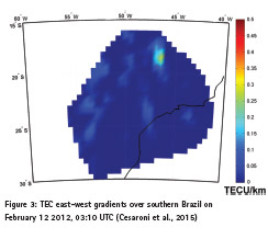
To further highlight the locations where ionization levels over neighboring sectors change the most, the TEC gradients can be used. Usually east-west and north-south TEC gradients are presented. Figure 3 represents such visualization, revealing the highest east-west gradients in the northeastern part of the observed region. That information can be useful to the users of differential GNSS or Ground Based Augmentations System (GBAS), as on locations with high TEC gradients the ionization levels for a referent receiver and an end user can be very different.
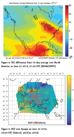
Even though TEC and its gradients provide very useful information, they lack the information on variability with time. Therefore, using only a TEC image it is not possible to conclude if the ionization levels change or remain the same, are the observed conditions usual for the area or not and are the disturbed regions moving or are they static. To answer those questions, TEC maps from different time epochs are needed. For instance, as presented on Figure 4, it is possible to observe the difference between current TEC values and its 10-day average. That difference reveals the areas of disturbed ionosphere and can indicate that single frequency GNSS receivers that rely on global ionospheric models will probably experience accuracy degradation in such regions.
In order to focus more on current ionospheric dynamics, Rate of TEC (ROT) can be used. ROT represents the amount of change of TEC in one minute. While TEC revealed the areas with the highest and the lowest ionization levels, ROT reveals the areas with the biggest change of TEC levels. Figure 5 shows ROT over Europe, calculated on points marked in red and interpolated in between. In non-disturbed ionospheric conditions the ROT values in middle latitudes are usually very low, but in depicted example a strong geomagnetic storm was underway, causing fast changes in ionization levels. The highest changes are observed in the northern part of the observed region, over Denmark, Scotland and Finland.
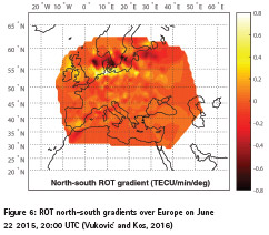
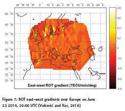
Spatial gradients of ROT can be calculated to show the trends in the ionospheric dynamics. The north-south gradients shown in Figure 6 are dominant in comparison with the east-west gradients shown in Figure 7, both reaching their maximal values in the area over Denmark. Over Scotland and Finland the ROT was high, but the levels increased gradually with distance and therefore the gradients remained low. In the areas with high ROT spatial gradients the neighboring regions experience different rate of change of ionization and the absolute values of TEC in these regions can also be expected to differ more in the following moments.
ROT Index (ROTI), a standard deviation of ROT during a 5-minute period can also be used to highlight areas with ionospheric irregularities, especially those smaller in size.
GNSS and ionosphere – Information cycle
Research communities in the fields of GNSS and ionosphere benefit of each other. GNSS are a powerful tool for ionospheric research, continuously providing data from around the world, with ever increasing number of available receivers. Public availability of the data and standardized data formats play key role in enabling ionospheric studies, comprehensive both in timespan and geographic coverage. The GNSS based ionospheric data can be further processed, creating TEC derived products which show the current state of the ionosphere, reveal its temporal dynamics and highlight the areas with the highest amplitudes of changes in ionization levels. Usually a combination of products should be used as they complement each other. Based on such GNSS-databased information the ionospheric models can be improved, the real-time data can be passed to the users and predictions on ionospheric conditions can be proposed. Finally, GNSS is the greatest beneficiary of better understanding the ionosphere, along with technology and business sectors relying on accurate GNSS based positioning, navigation and timing (PNT).
Acknowledgment
The research leading to these results has received funding from the European Community’s Seventh Framework Programme (FP7/2007-2013) under grant agreement No. 607081.
References
Cesaroni, C., Spogli, L., Alfonsi, L., De Franceschi, G., Ciraolo, L., Galera Monico, J. F., Scotto C., Romano, V., Aquino, M. and Bougard, B., (2015), “L-band scintillations and calibrated total electron content gradients over Brazil during the last solar maximum”, J. Space Weather Space Clim., 5, A36. doi: 10.1051/swsc/2015038
NOAA/Space Weather Prediction Center, “Real-time US-Total Electron Content: Vertical and Slant – Difference from 10 day average indicating recent trend”, Accessed on June 23 2015. http://legacy-www. swpc.noaa.gov/ustec/DIF_index.html.
UNAVCO Inc., “Data Archive Interface v2”. Accessed on June 6 2017. http:// www.unavco.org/data/gps-gnss/dataaccess- methods/dai2/app/dai2.html#.
Vuković, J. and Kos, T., (2016), “Ionospheric spatial and temporal gradients for disturbance characterization”, Proceedings of 2016 European Navigation Conference (ENC), Helsinki, pp. 1-4. doi: 10.1109/ EURONAV. 2016.7530564.


 (No Ratings Yet)


Leave your response!