Earthquake analysis by 3-D affine deformations

James L Farrell VIGIL Inc., Institute of Navigation Pacific PNT 2013, Honolulu Hawaii, USA

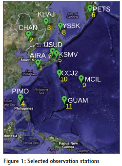
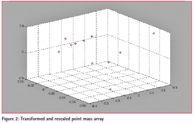
In this first application of morphometrics to earthquakes, plot sequences are first provided for coordinate shifts, rotations, and uniform scaling on each separate day. In addition to those seven time histories from Procrustes representations, five more offer further insight: shape states (three shear and two nonuniform scaling). For those, classical (two-dimensional; ‘2-D’) methods from anatomy had to be extended to 3-D. All were obtained for landmark coordinate sets reported daily for four weeks before and after the 2011 Tohoku quake. Findings exhibit encouraging prospects for anticipation, in time and spatially. Data provided herein enables readers to verify sample results.

Introduction

An illustration of the methodology used here is available from selected station location histories before and after the Tohoku quake in 2011. Figure 1 shows the chosen stations on a map [1] and Figure 2 depicts them following rotations and normalizations to be described herein. The eleven stations are represented as a 3-D structure consisting of point masses all tethered to their collective centroid by weightless connecting arms that are not quite rigid. With migration the centroid shifts accordingly while the connecting arms rotate and deform to accommodate as necessary. Migration irregularities preclude exact mathematical characterization for the pattern of accommodating adjustments, but a daily affine transformation sequence serves as a useful model for analysis and interpretation – with prospects for anticipating earthquakes in the future.

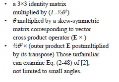
Background from related fields

Methods from branches of multiple disciplines are highly relevant. For this first 3-D affine deformation analysis applied to earthquakes, presentation calls for recognition of pertinent sources. At the same time, their descriptions here cannot exceed length restrictions. A full mathematical development, accompanied by the complete set of results to be shown, would violate length limitations. Alternatively that development, without the results, could cause readers to feel “lost in a sea of equations” with any potential benefits yet to be seen. Complex equations are therefore absent from this paper; methods are described verbally in reasonable detail but, for derivations, heavy reliance is placed on selected references. For ease of familiarization, applicable reference material is focused as narrowly as permissible. Wherever possible, verbal descriptions are worded so that the reference will not be needed by those familiar with material being discussed.

Mathematics

Developments of standard tools itemized in this subsection, including derivations, are available from many sources. Major operations include 1) minimum variance estimation, 2) coordinate rotations, 3) diagonalization of 3×3 square matrices, 4) singular value decomposition (svd) of rectangular matrices, and 5) 4×4 affine transformations.

Coverage of the first three items, with some subtle features needed for this specific application included, can be found in [2]. With usage of the block (rather than sequential) estimation, the brief development on pages 159-162 suffices. Even that is more general than needed for the steps followed here (though not for recommended future extensions). Pages 36-38 of [2] cover 3-D coordinate rotations, but that latter page shows a popular small-angle representation acceptable in most operations – though not used here. When rotating vectors of enormous size (hundreds of km), adequate precision must be ensured. Here that translates into approximating the cosine of a small angle – not by unity but by a two-term representation. A direction cosine matrix that rotates through a small angle θ about any axis with unit column vector , contains three ingredients:

.

Another transformation involves reexpression of latitude/longitude/altitude into earth-centered, earth-fixed (ECEF) coordinates. Again the operation is standard; those unfamiliar can examine Eq. (7-31), with (3-18, -19, -22), of [2]. Also the inverse is described in addendum 5.E of [3]. Diagonalization of a square matrix is defined in [2] by Eqs. (II-20, -21, -22), with examples given in pages following them. Standard algorithms are common, e.g.,

[evec, eval] = eig(matrix)

in MATLAB. For matrices that are rectangular rather than square a related operation (svd) is used: adequate for purposes here, again from MATLAB,

[M_U, D, M_V] = svd (U V^T)

The role of the eigenvector matrix denoted “evec” plus the factors denoted M_U, M_V, U, and the transpose V^T of V, are defined in subsections that follow.

Affine transformations, central to this investigation, offer a much wider scope of effects including translation, scaling, and deformation as well as rotation. The standard 4×4 affine transformation in 3-D, being homogeneous, has one less independent state than the number (sixteen) of matrix elements. The fifteen independent states can be categorized in five sets of three, each set having x-, y-, and z-components for translation, rotation, perspective, scaling, and shear. Immediately the three degrees-offreedom associated with perspective are irrelevant for purposes here. In addition both translation and rotation, clearly having no effect on shape, can be analyzed separately – and the same is likewise true of uniform scaling. It is thus widely known that there are five “shape states” involved in 3-D affine deformations, three for shear and two for nonuniform scaling.

One way to describe shape states is to note their effects in 2-D, where there is only one for nonuniform scaling (which deforms a square into a rectangle) and one for shear (which deforms a rectangle into a parallelogram). Therefore it is suggested here that added insight into earthquake investigation can be obtained by analyzing affine features – with specific attention given to their individual traits (degrees-of-freedom).

For those unfamiliar with affine matrixes, [4] provides an excellent thorough introduction plus numerous examples. Due to their central role, they will appear repeatedly in multiple discussions to follow.

Anatomy

Familiarization with the topic now to be broached sometimes begins with the example of facial features (e.g., tip of chin, corners of the eyes and mouth). Those qualified, however, identify landmarks on other anatomical structures for further study (e.g., as a possible diagnostic tool if certain deformations correlate with some affliction). When measurements (e.g., from x-ray images) are processed as described shortly, specific landmarks – even from a wide variety of patients (any nationality, any race, all ages, both sexes) – are found to cluster with some degree of consistency. That trait is physiological, not an artifact of the processing. Also, when the landmarks are remapped after extraction of affine deformations, the clusters shrink; theoretically if only affine deformations were present, clusters would converge to discrete points.

The universally recognized reference [5] contains thorough descriptions of the entire process plus a wealth of results, along with a full derivation (from pages 138-142) developed by the author of [6] for affine deformation states – all in 2-D. Needless to say this presentation will not include that derivation, let alone its 3-D extension. What can be realistically offered here will nevertheless enable partial application of this methodology to other data sets, with or without this author’s involvement. Not all of the results to follow require the complete deformation analysis. In generating those results, some very revealing features arose in earlier portions of the overall procedure – without requiring full pursuit to final determination of 3-D deformations. For this data set, at least, understanding can thus be brought to a significant level with just the Procrustes representation, described succinctly as follows:

The previously defined structure of K point masses and nonrigid connecting arms (K = 11 in this study) is first transformed into principal axes of inertia (next subsection) and the origin is translated to the centroid. Division by the root sum square of all coordinates then produces an array containing 3K dimensionless positive and negative numbers whose sum of squares is unity.

With normalization of all magnitudes an orthogonal matrix, computed for each separate day of the sequence, minimizes that day’s sum of squares of rotated landmark changes from the first (“Day #I”). It is formed, as on page 98 of [6] but with notation modified here, as a product M_V M_U ^T of outer factors from svd with U and V, 3×K matrices produced by the set of Procrustes operations just defined, acting on the data from Day #I and each subsequent day, respectively.

After forming all Procrustes coordinate matrices and storing columns of U into vector , affine transformation provides an array u of small adjustments for each day’s fitted array , nominally characterized as +. Explanation is now in order, due to differences from applications to anatomy. Here there is no need to form an average mesh; Day #I’s coordinate set serves as the comparison reference throughout. Also the coordinate adjustments, shape states, and rotations from svd here are are not merely small; they are minuscule – of order 1.e-8. Still the need for precision calls for rigorous computations; over a span of 1000 km, 0.01 µradian rotations generate cm displacements. Even withorthogonal toan adjustment is made; u is summed – not with but with / |+ | – see next subsection.

Also of potential interest from the field of anatomy are further deformations represented by a thin plate spline (TPS, which minimizes approximate squared curvature integrated over a surface defined by a landmark set). Nonlinear (unlike affine) deformations are applicable over only local regions rather than entire structures. Full implications of that issue, quite broad in physiological studies, involve complex topics not needed for this landmark analysis (e.g., sophisticated mathematics of Riemannn manifolds and the impact on detailed algorithms for dense correspondence in positioning pixels between landmarks of high resolution images). For this application only the TPS is considered – and only briefly, at that – since results obtained show that variations in the dayto- day bending energy obtained from it are negligible for practical purposes. Mechanics Only a few concepts from this branch were used here. It was foreshadowed earlier that adding a miniscule vector orthogonal to a unit vector must not result in a significant length increase. That “arc length constraint” is modified somewhat here; more generally, although the affine deformation vector u can include expansion/contraction effects, no artificial elongation is introduced through vector addition (hence division of U by |U+u |). Although that same principle theoretically applies to the TPS (which equates curvature to a second derivative without the slight shortening just described), that adjustment has not been found necessary (nor feasible) for TPS fitting.

Their sum is the matrix to be diagonalized, described earlier.

Strength of Materials

Deformations have spatial derivatives in along-axis and across-axis directions. The latter, in order, are associated with slopes, components of curvature (proportional to bending moments), and curvature gradients (proportional to shearing stress) while along-axis deformations (extension and contraction) are related to tensile and compressive stress. In-depth pursuit of these and other additional forces (e.g., friction) would clearly involve still another field of endeavor, i.e., geology, to take into account tectonic plate characteristics (composition, inhomogeneity, irregular cross-section geometry, elasticity, etc.). Although beyond scope here, a limited effort toward that direction was originally intended, by using an available TPS program. The program did quantify bending energy but, at least for the period of primary interest (pre-quake), those temporary elastic deformations lowered that priority for the data studied. Reasons are traceable to the diminutive changes in coordinates compared to the distances spanned. Dominance of other factors would not justify further emphasis on nonlinear deformations.

Procedure

A synopsis of steps summarizes the preceding descriptions:

• select an ensemble of station histories to be analyzed
• acquire data in most reliable and accurate form
• assemble coordinate data into arrays to prepare operations
• use each separate day’s landmark set centroid as origin
• form the inertia matrix of the first day’s landmark set
• diagonalize the inertia matrix for principal axis resolution
• form a direction cosine matrix from the eigenvectors
• shrink each day’s centered landmark coordinate sum of squares to unity (this step could either precede or follow the next)
• transform each day’s landmark data set through the 3×3 orthogonal matrix
• rotate again per svd from each day’s data vs Day #I
• compute estimates for each day’s five shape states
• apply shape states to the reference (Day #I) data
• backtrace steps to reconstruct input data; evaluate the fit based on residuals
• prepare all results for dissemination/presentation

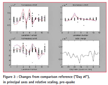
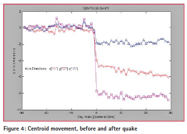
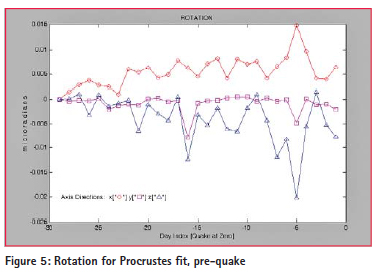
Completion of all steps can enable interpretation and evaluation of outcome as means for quake prediction. Toward that objective, recommendations for further tasks to be pursued follow the results now to be presented.

Quantitative results

Disturbances appearing in advance are seen from plots using an abscissa indexed with the quake at zero. From data files starting 29 days prior, then, “Day #I” is indexed at -29.

Each x, y, and z landmark migration in Figure 3 appears as a single dot, except for those depicted by two solid lines used to show some deviations from general patterns. Occurring five days and sixteen days before the quake, they are somewhat more pronounced in the lower right plot. Further changes after the quake are of course larger, but higher priority is attached here to pre-quake behavior.

While early disturbances are entirely consistent with past experience, processing the data in another way can lend further insight. Here the changes are reexpressed in terms of the deformed Procrustes representation used for this study. To begin that portrayal, pre- plus post-quake centroid shifts and prequake small rotational adjustments are shown in Figure 4 and 5, respectively.

The permanence of change in Figure 4 is obvious and not at all surprising. Again the foreshadowing at 5 and 16 days prequake are detectable, and of course would be more clearly visible on a half-duration plot (i.e., terminating one day before the quake, as Figure 5 does for the rotational history). The last two plots offer some added premonitions. The temporary character of these advance disturbances (tendency to return toward earlier forms) is suggestive of elastic deformations, but

• only a partial restoration occurs, and
• there is some growth of deformation peaks.

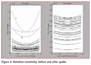
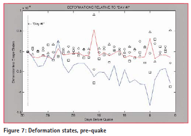
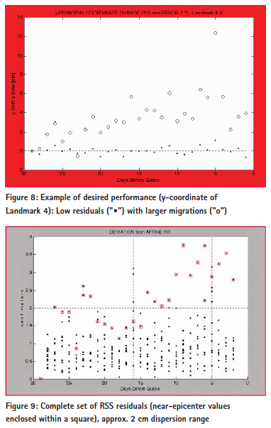
Issues just noted are revisited in later sections. First it is of interest to follow through with additional behavior patterns, starting with a serendipitous clue that arose while validating the small-angle rotations of Figure 5.

Formation of the orthogonal matrix with the outer factors from the svd, as previously described, was first shown to provide the minimization as promised. That verification produced Figure 6, now described as follows: Separately in sequence, centroids of each day’s K landmark appendages colocate with that of Day #I. Migration nonuniformity precludes coincidence of point mass extremities but the sum of squared separation distances is minimized by the orthogonal matrix from the svd. Multiplying the angle through a span of values (from too little to too much rotation) always made the closest combination for a multiplier of unity. Generally the sum of squares tends to grow as the quake draws near (except for the same days already noted and also one day ahead. No definitive diagnosis will be attempted from this amount of data, except to say that the phenomenon warrants wider investigation.

As one step toward wider scrutiny, sensitivity to the rotation axis direction was also determined. Resulting 3-D images for 29 days cannot be plotted together without masking each other, but the outcome is similar. The three days noted in Fig. 6 exhibited abnormal sensitivity to the direction, as well as the amount, of rotation. Furthermore, also on those same days, at least three shape states (not always the exact same set) temporarily jumped beyond their normally moderate growth trend. Before switching attention to the shape states, it is noted that behavior of this data set is not guaranteed to hold in general. Other attributes could arise from chosen landmark sets with dissimilar layout geometries (or even from an alternative choice of shape states for this data set – recall that there are two expansion / contraction states covering three directions). These points facilitate understanding Figure 7 but, again, no generalization will be attempted here; data from other quakes could show different behavior.

Figure 7 is seen to be consistent with discussion preceding it, while exhibiting numerical values comparable to the rotation states of Figure 5. Also, local pre-quake peaks are again apparent in the expansion / contraction state line plots and the symbols representing shear states. Immediately a question can arise, regarding conformance of this model to migrations actually observed. Numerous plots vs time and vs landmark number, made to evaluate that conformance, are discussed next.

Coordinate plots computed from the model, together with actual observations, seem impressive but not informative (points “coincide” when migrations are dwarfed by distances between landmarks). Alternatively a migrations-only plot, showing departures of modeled from observed values, exhibit the limitations more clearly – but without indicating what constitutes “good” performance. Figure 8 exemplifies the information desired by showing migrations actually observed together with errors in modeling them.

The total volume of data (in three directions from eleven landmarks over a period of weeks) necessitated a way to compact the results for this affine model. That effort, applied to RSS values (3-D x, y, z), produced Figure 9 described as follows: Most residuals (shown with a dot • ) fall very near or below the dashed horizontal line at 2 cm. Exceptions are

• values obtained at 16 and 5 days prequake (the main “early warning” days, light dashed vertical lines)
• landmark #5 (closest to the epicenter), whose residuals are enclosed within a square
• two others (shown encircled) at about 2.2 and 2.6 cm.

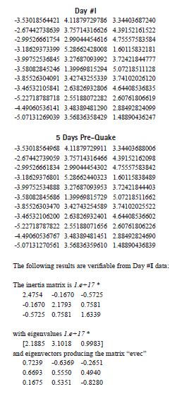
To reiterate, all residuals are below 4 cm., almost 98% are below 3, and over 91% are below 2. All but two of the values significantly above 2 cm are either from the station nearest epicenter or from one of the key early warning days.

With 3-D RSS migration reaching a maximum of almost 15 cm amidst dispersions of a few cm, these results are consistent with performance expected from minimum variance estimation. By analogy with a straight line or low order curve fitted to scattered empirical data, a least squares fit here captures the larger migrations while accepting residuals commensurate with the dispersion in the data.

Some further discussion of these residuals is warranted. The plot of this full set in Figure 9 was preceded by a partial glimpse (Figure 8), in one of three principal (not ECEF) axes from one of eleven landmarks. Few partial plots look as good as that sample. For landmarks with smaller migrations (4 or 5 cm maximum), a nominal 2-cm dispersion is less impressive – and individual excursion components from some landmarks were in fact less than 2 cm. What those cases contribute, to be blunt, “just looks like a bunch of dots thrown all over the place.” A fitted model will not adhere to the points. Attempts to force model fidelity are readily dismissed; many will recall MATLAB’s “doomsday” polynomial fitted to empirical global population history.

Model credence for data analyzed here rests on acceptance of 2-cm residuals as a reasonable (though admittedly not trivial) price to pay for a means of characterization. Immediately a caveat might be raised: Shouldn’t that be changed – contingent on acceptance of 4-cm residuals? Actually no; aside from the two circled points in figure 9 (beyond 2 cm by modest amounts), the “problem” of larger residuals is in reality the opposite of a problem. They offer valuable revelations, in time (premonitions at 16 and 5 days pre-quake) and spatially – most of them correspond to the landmark closest to epicenter! As with other facets of this investigation, no generalization will be attempted – but other quakes should be examined for these traits.

Data for verification

As promised, data will now be included to enable duplication of certain results – and subsequent application to observations from other quakes. A full data set, even from the limited scope of this study, would be unwieldy – but coordinates at Day #I and at five days prequake allow revealing traits to be exhibited. Those values, in centimeters, are obtained through multiplication by 1.e+8 the next two tabulations for x, y, and z:

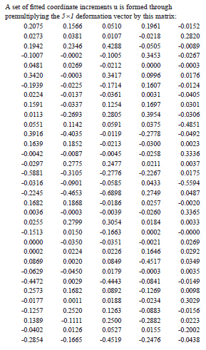
From both days’ centroid-referenced coordinates the svd produces a small-angle rotation vector equal to 1.e-7 * [.14830897738546 -.04830307526257 -.20219407067329] which together with principal-axis rotation via “evec” enables validation of the top curve on the left of Figure 6. Additional data will now be presented to enable an accuracy evaluation for the affine fit to the preceding tabulation of pre-quake coordinates. The deformation vector obtained for that day was the product 1.e-9 multiplied by [-0.456365 -5.20928 4.77305 3.19895 -13.2300]

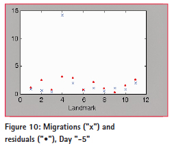
The accompanying plot shows, in cm, RSS migrations and backtrace-reconstructed coordinate residuals in ECEF.

Figure 9’s largest residuals, “BTW” encouragingly, occur at a landmark other than that with largest migrations. Also, RSS migrations and reconstructed coordinate residuals in principal axes rather than in ECEF produced subplots somewhat (but not dramatically) better than Figure 10. From material already presented it could be anticipated that

• individual (x, y, and z) components exhibit some traits that are more impressive (small residuals with relatively large migrations) and some that are less so (migrations and residuals both near 2 cm).
• the former are reminiscent of Figure 8 while the latter call to mind the “bunch of dots” perception.

Many other plots were generated whose presence here might add only marginally to material already shown. Post-quake time histories, for example, show poorer adherence to affine modeling – even with the “Day #I” reference moved to the first day after the quake. Additional prospects, seeming to warrant further attention even pre-quake, were noticed but not yet fully pursued. Of primary importance at this stage of presentation is a clear understanding of what the affine fit – based on evidence obtained thus far – offers toward quake anticipation. In brief, the least squares fit appears to

• provide awareness of the larger landmark excursions while “middling and muddling through” the smaller and, in the process of doing that,
• suggest clues in advance regarding time and location

Limits of time and space now prompt a shift of attention to listing of areas deserving extended investigation.

Recommended future extensions

Insight gained thus far easily justifies advocacy for accumulating a data base from experience, by applying morphometrics to several more known quake histories. That recommended effort could employ both variations in, and extensions of, methods used here. The former (i.e., variations) could include assembling data blocks with modifications in content. While an increase in station density has obvious practical limitations, there could be multiple runs with different station selection criteria (based on association with tectonic plates, full encirclement of epicenter, etc.). Measurement count could be increased by longer pre-quake duration, higher measurement frequency, and/or integration [3] with a low cost IMU for short term motions. Also it must be recognized that errors in recorded coordinate values are correlated (above-horizon geometry alone is sufficient to guarantee that) – but they are processed as if they were independent. The way to quantify that effect is to record individual satellite measurements instead of coordinates [7] with weighting based on (potentially nonuniform) individual measurement accuracies.

Extensions of procedures used herein could account for

• alternate shape state formulations, with other pairs of axes chosen to have the independent expansions
• strength of materials (bending for shear states, tensile and compressive strength for expansion / contraction)
• inhomogeneous tectonic plate composition, irregular cross-section geometry
• other items (static friction, partially abutted surfaces • • • ).

Other possible extensions, probably with lower priority at present, might include pursuing the TPS further, addition of deformations with spatial nonlinearities (i.e., nonlinear only w.r.t. position but not nonlinear w.r.t. the state – in analogy with linear estimation for a quadratic or cubic polynomial fit), or other non-affine deformation patterns (e.g., twist). In any case, highest value will be attached to models showing consistency with empirical quake data, and experience gained from analyzing past histories will offer predictive capabilities for the future.

Further promising applications (with suitable modification): tsunami prediction [8] and aging infrastructure.

Conclusions

For investigation of earthquakes based on their affine degrees-of-freedom, methodology of another field –anatomy – is highly relevant. Instead of designated landmark sets coming from a group of patients, here they are associated with a series of days (e.g., from several days before to several days after a quake). Each landmark set is then subjected to a sequence of procedures thoroughly familiar to anatomy experts and succinctly reviewed herein.

Physiological studies of affine deformations in current practice ironically lack a crucial feature; they concentrate heavily on two-dimensional representations. While full affine representation is very old, its inversion (i.e., optimal estimation of shape states from a given overdetermined coordinate set) has heretofore been limited to 2-D. Immediately then, extension was required for adaptation. The fundamentals still remain applicable, however, as indicated by several plots presented in this paper.

A serendipitous discovery, verifiable from data included here and easily applied to other quake histories, calls for further investigation. Sensitivity to incremental rotations, formulated from Procrustes representation even without computing affine deformations, jumped beyond range before returning to “normal” – twice, well in advance of the quake (i.e., first by sixteen days and Figure 10: Migrations (“x”) and residuals (“•”), Day “-5” subsequently by five days). That behavior, plus other results shown herein, exhibit encouraging prospects for warnings in advance of quakes (and potentially, tsunamis or infrastructure failures).

Acknowledgment

Prof. Frank van Graas and Ryan Kollar of Ohio University provided all landmark data for this investigation. Without their diligent acquisition and validation of the data, none of the results presented here could have been generated. They join me in appreciation of the opportunity to pool our efforts with others in this field, toward reducing the danger to those ar risk from earthquakes.

References

[1] F. van Graas and R. Kollar, “Processing of GPS Station Data for Prediction Algorithm Analysis of the 2011 Tohoku Earthquake,” ION Pacific PNT 2013.

[2] J.L. Farrell, Integrated Aircraft Navigation, Academic Press, 1976 (now in paperback; – http:// jameslfarrell.com/published-booksgnss- aided-navigation-and-tracking

[3] J.L. Farrell, GNSS Aided Navigation and Tracking, Amer. Literary Press, 2007 (http://jameslfarrell.com/wpcontent/ uploads/2012/03/GPSINS.pdf).

[4] D.F. Rogers and J.A. Adams, Mathematical Elements for Computer Graphics (2 ed), McGraw-Hill, 1990.

[5] M. Zelditch et. al., Geometric morphometrics for biologists: a primer, Academic Press, 2004, ISBN 0-12-77846-08, pages 137-142.

[6] F. Bookstein, “Shape and the Information in Medical Images: A Decade of the Morphometric Synthesis,” Computer Vision and Image Understanding, v66 n2, May 1997, pp. 97-118.

[7] J.L. Farrell, E.D. McConkey, and C.G.Stephens, “Send measurements, not coordinates,” ION Journal, Fall 1999, pp. 203-215

[8] R. Nakasone and N. Kubo, “New Approach for Tsunami Detection Based on RTK-GNSS using Network of Ships,” IONGNSS- 12, Nashville TN, 2012.