| GNSS | |
Stochastic behaviour quantification of GNSS receivers
In this paper, the repeatability standard deviation has been defi ned and measurements have been performed |
 |
|
 |
|
 |
|
 |
|
For intelligent transportation systems the information of any vehicle location in an absolute geodetic reference frame is essential. These locations can be estimated best on the basis of global navigation satellite systems combined with auxiliary sensors. A GNSS receiver serves as the major component. Since more and more GNSS are available or will be built up in the near future, availability and accuracy will increase. Therefore, the reliable determination of the receiver quality is currently under research at multiple institutions e.g. [1]. Especially for GNSS system manufacturers and system integrators, it is essential to determine which receiver is the most suitable for their specific applications. Thereby, the field performance evaluation is mostly performed by static tests or by kinematic tests driving randomly through an urban environment. But the gathered data is only a snapshot of the receiver performance and has a lack of statistic significance.
Measurements have shown that GNSS receivers of the same type with identical software versions and software settings provide different location data [2], even when operated with the same antenna input signals. That phenomenon has multiple reasons: maintaining a digital phase lock loop is a very stochastic process especially in dynamic scenarios, receiver clocks are strongly temperature dependent and some parameters of internal filters have an internal memory effect [3]. Two examples are depicted in Figure 1.
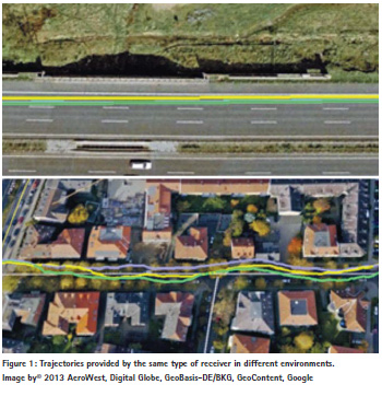
The images present different trajectories of three GNSS receivers of the same type and same software versions, provided with the same input signals. It is visible that on the highway scenario (above) the distances between the trajectories are much smaller than in the urban scenario (below). This leads to the result that for a liable performance assessment it is not sufficient to execute simply one or few tests to estimate the performance parameters reliably. To deal with this situation, a new parameter has to be defined to quantify the repeatability characteristic.
Until today, there are mainly two options for testing the GNSS receiver and antenna combination on their stochastic behaviour. They can either be tested in parallel resulting in a large amount of receivers or one receiver can be provided with the same signals (recorded by a record and replay system) repeatedly. To provide a receiver with real signals, they have to be recorded during a test run and afterwards replayed in the laboratory. That operation can be performed with signal record and playback systems through the originally installed antenna. These systems work in the way that active GNSS signals are filtered, amplified, down converted and digitized. Later, in the laboratory the data can be replayed by reversing the process. In contrast to field tests, the financial cost of test repetitions is low. Hence, such a system is used in this paper to investigate the stochastic behaviour.
Methodology
Typical key performance accuracy characteristics such as trueness and precision (variance resp. standard deviation) are calculated according to the general understanding in metrology as the evaluation of the difference xi between a reference location xr,i and the measured location xm,i (see eq. 2) [4]. To investigate the stochastic behaviour of the system under test, a new quantity, called the repeatability standard deviation, is introduced. That measure quantifies the standard deviation of possible location deviations from signal replays by means of the standard deviation for a scenario. This measure is derived from ISO 5725 where the repeatability is expressed by the repeatability variance. There it expresses the quality of a measurement system operated in different test laboratories [5]. In contrast to variance, standard deviation is a measure of dispersion which is much more illustrated. Therefore, the repeatability in this paper is presented by the repeatability standard deviation of the quantity introduced at the beginning. If the repeatability standard deviation is large, a strong stochastic behaviour with large standard deviations between different measurements is visible. If the repeatability standard deviation equals the standard deviation of the corresponding true measurement, the system reveals with a high probability a deterministic behaviour. The repeatability standard deviation sr is formulated as:
![]()
with sij being the variance of the performance parameter j of replay i, nij the amount of samples in replay i of performance parameter j, and p the total amount of replays. For reasons of simplicity, the index for the different scenarios is not included in eq. 1. Before calculating the repeatability, the measurement samples have to be investigated in terms of outliers. One possible test advised by ISO 5725 [5] is the Grubbs’ test for outliers. At the beginning of the test, the mean location deviation:

with xi being the measurement value of a test, P the amount of measurement samples, the mean value of all measurements and s the standard deviation of all measurements. This is followed by the comparison of GP and the critical value for Grubbs’ test α , calculated from the student-t distribution or extracted from tables. If GP > α , an outlier is detected, the value has to be excluded from the sample and the test has to be redone with the newly calculated values. If GP < α , no outlier is detected and the repeatability standard deviation can be calculated.
Lastly, the confidence in the measurement results is of interest. It can be expressed by a confidence interval. This confidence interval defines a range around the mean value, where the real mean will most probably be. The confidence interval CI can be calculated by:
CI = 2 · SE · z (5)
In this equation, SE stands for the standard error of the sample mean and z the quantile of the distribution. For this case a normal distribution is assumed and a 95% confidence is chosen. Hence, for the following calculation 1.96 is used for z. The standard mean error can be calculated for a given standard deviation s and the total number of samples for all replays n by:
![]()
Test data acquisition
To quantify the repeatability standard deviation, both real test data and replayed test data are required. During testing, the antenna was mounted on top of the test vehicle. From there signals were transmitted via a 0 dB antenna splitter to a reference measurement system, the GNSS receivers and the record and replay system. The reference measurement system was an INS system manufactured by OxTS provided with real time correction data from a certified local reference data provider. The reference locations of the reference system are known to be accurate to cm level. Hence, it can be regarded as the true value for this type of application. The systems under test were provided with the same signals at all times. During the test, measurements were performed with two Ublox Neo- 6P GNSS receivers. All receivers were configured for the automotive application and to use SBAS data. To collect the necessary data for calculating the repeatability standard deviation, a record and replay system Spirent GSS6425 was carried along. It supports 3 frequencies, enabling the recording of GPS, GLONASS and SBAS data. Whereby, GLONASS data was not analysed.
To analyse the impact of the environment on the repeatability standard deviation, different scenarios have been classified in terms of the type of street, the height of surrounding buildings and their distances to the streets, the occurrence of highly reflecting materials and possible signal degradation elements such as trees. The urban scenario with trees comprises for example high buildings close to the street with trees growing between buildings and the street.
Results
The results contain the evaluation of both i) the real measurement (August 2015) and ii) the replayed measurement data. To calculate the accuracy for both types of data, the coordinates provided by the reference measurement system were used.
Evaluation and results of real measurement data
First the location deviation in terms of trueness and standard deviation is calculated. Therefore, the difference of the reference location and the measured trajectory is calculated, followed by the calculation of the mean location deviation and standard deviation for each scenario. The location deviations for the different scenarios are depicted in Table 1.
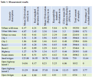
It is obvious that the scenarios show major differences for the mean location deviation for the different environments. One very interesting result is that the ‘Rural 1’ scenario has the lowest mean location deviation, but the most precise scenario is the ‘City 1’ scenario. The special scenarios (bridges and tunnels) surprise with high location deviations. This is due to the very challenging environmental conditions. The steel bridge scenario e.g. is the most limiting scenario, where the line of sight signal reception is completely denied.
Evaluation and results of replayed measurement data
After the test drive, a total of 11 replays was performed and recorded. In a first step, the replayed measurement data as well as the real measured data were analysed. In a second step, the measurement sets were analysed for outliers. Once all outliers were excluded from the measurement, the repeatability standard deviation was calculated according to eq. 1. The results for the real and the replay measurement data are concluded in Table 1.

At first glance the mean deviation between the true measurement and the total mean of the replayed signals exhibits strong variations. This is strongly depending on the environment. It can be seen that open environments such as ‘Highway’, ‘City 1’ or ‘Rural 2’ differ in the range of decimetres. In contrast, for more sophisticated environments the mean location deviations differ in the range of meters (urban scenarios) to multiple meters (forest, steel bridge)
The repeatability standard deviation demonstrates the stochastic behaviour of the GNSS receivers under test. But there are strong differences between the different scenarios. For scenarios with low mean location deviations, the repeatability standard deviation is low. In contrast, it can be seen that for scenarios with large mean location deviations the mean standard deviation is also large. This behaviour is depicted in Figure 2, where the two extreme scenarios ‘Steel bridge’ and ‘Open highway tunnel’ are left out. It can be identified that there is nearly a linear behaviour with a degression towards higher values of the repeatability standard deviation. This observation leads to the fact that it can be assumed that in challenging environments the stochastic behaviour is more distinct than in open sky scenarios.
The confidence in the measurement is expressed by the confidence interval. It can be seen that for 11 replays the confidence interval differs for the scenarios. For some scenarios, the true mean lies most probably within 1 meter, for others the confidence is much smaller. To get reliable results, more replays are required, at least for the more complex scenarios.
For some scenarios, the total number of outliers is quite high, but only limited strugglers were identified. Most of the outliers have their origin in a replay performed within the moving vehicle. It is assumed that due to vibrations of the vehicle the internal clock of the replay system was disturbed. The exemplary Grubbs statistic G is depicted in Figure 3. In this figure, G values of repetition 3 exceeds the α values clearly for a certain time.

The behaviour of larger location deviations for that replay is visible when the trajectories of each trip are plotted in Figure 4. It can be seen that repetition 3 (large position deviation at the beginning) does not follow the other repetitions. Even though one imperfect replay was identified, the maximum amount criterion of outliers according to JRC 51300 [6] (exclusion of maximum 2/9 of the samples) is still fulfilled.
Conclusion
In this paper, the repeatability standard deviation has been defined and measurements have been performed.
With the conducted measurements it could be proved that it is not sufficient to simply go out into the field, drive around and acquire measurement data. Within the measurement results, strong variations were even visible for the mean location deviation. Furthermore, it could be identified that the measurement environment has a major impact on repeatability.
Depending on the system under test and the environment, the repeatability standard deviation varies strongly.
Hence, to achieve reliable results and to consider the stochastic behaviour, multiple measurements with the same input signals have to be performed. That can either be done by testing different systems in parallel or by using a record and playback system. For the measurement results presented, the confidence intervals were calculated. By increasing the number of replays, the confidence range could even be reduced. One open question is the impact of the record and playback system quality on the measurement results. This is currently under investigation.
Acknowledgment
This research was supported by the International Science & Technology Cooperation Program of China (2014DFA80260). This paper was already presented at the European Navigation Conference 2016 in Helsinki.
References
[1] D. Lu and E. Schnieder, Performance Evaluation of GNSS for Train Localization. In: IEEE Transactions on Intelligent Transportation Systems, No. 90, 2014.
[2] D. Spiegel, F. Grasso Toro, E. Schnieder, A Satellite Independent High Dynamic Test Bed and First Measurement Results, in: Proceedings of the 27th International Technical Meeting of The Satellite Division of the Institute of Navigation (ION GNSS+ 2014), September 8 – 12; pages 433 – 439, 2014.
[3] E. Kaplan, C. Hegarty: Understanding GPS Principles and Applications: Principles and Applications. 2. Ed. Artech House, Norwood, USA, 2005.
[4] M. Wegener, ”Über die metrologische Qualität der Fahrzeugortung”, Dissertation, Institute for Traffic Safety and Automation Engineering, Technische Universität Braunschweig, Braunschweig, Germany, 2013.
[5] International Organisation for Standardization: ISO 5725-2:2002: Accuracy (trueness and precision) of measurement methods and results, 2002. [6] Joint Research Centre (European Comission): JRC 51300:Area measurement validation scheme, Technical Note, Luxembourg, 2009.


 (No Ratings Yet)


Leave your response!