| Mapping | |
Mapping India on large scales – A quick and viable solution
A simplified approach for GPS assisted densifi cation of leveling network
|
 |
|
India was one amongst the few countries – including the advanced ones – to have completed topographic mapping on 1:50,000 and 1:25,000 scales, employing photogrammetric techniques, about four decades back. Since then there has been a tremendous progress in the field of Imaging and Geomatics by way of Global Positioning System (GPS), Inertial Measuring Units (IMUs), Large-Format High-Resolution Aerial Digital cameras, etc. Due to these developments, quite a few countries have standardized the scales as large as 1:2,500 and 1:1,250 for country-wide topographic mapping, and even larger scales ranging from 1:240 to 1:1,200 for engineering applications mainly due to operationalization of GPS, IMU and Digital cameras resulting in nearly complete automation in various photogrammetric processes, viz., aerial triangulation, Digital Terrain Model (DTM) / orthophoto generation, etc. The main advantage accrued due to these advancements is that there is a very little requirement of plan as well as height ground control points (GCPs) for photogrammetric aerial triangulation (AT).
It is well established that with aerial imagery flown with GPS / IMU for photogrammetric applications, GCPs are required only at the corners of the photogrammetric block. Whereas, if aerial imagery is flown without GPS/IMU, full (plan + height) control points are required at close intervals along the periphery of the block and height control points at much closer intervals in every flight line.
The provision of control points along with ellipsoidal heights is an easy task because these can expeditiously be established with the help of GPS. But height control points, also known as Bench Marks (BMs), are invariably required with heights above Mean Sea Level (MSL) and, therefore, cannot be determined by GPS.
Especially in countries like India, that have not yet established their own geoid, the only method available to determine the heights above MSL, known as Orthometric heights, is by means of precision leveling that is cumbersome, slow, costly and prone to errors. Some countries like US and Canada have established their own precise geoid along with a correction surface and have made the facility available to public for conversion of GPS (ellipsoidal) heights to Orthometric heights. The correction surface is generated from a sufficiently dense network of GPS control points and height BMs established by precise leveling.
Geomatics Center Canada provides an online facility for direct transformation of NAD83 or ITRF ellipsoidal heights of any point in Canadian territory to CGVD28 Orthometric heights, (CSRS-A). The National Geodetic Survey (NOAA) of US have released the GEOID96 (recently upgraded to GEOID12A) hybrid Height Model for Conversion of GPS Heights to NAVD88 Orthometric elevations, (Milbert and Smith, 1996). Facilities are available online for interactive computation of Orthometric heights from GPS ellipsoidal heights, (NGS Geodetic Tool Kit). Because of these facilities, these countries are able to take full advantage of the recent developments and carry out large-scale photogrammetric mapping most economically in a much smaller time-frame as compared to others who don’t have such a facility.
India is one amongst such countries who have not yet established a precise geoid along with the required correction surface. As a result, though India has the capability of acquiring aerial imagery employing most-modern digital cameras equipped with GPS / IMU, the requirement of plan and height control points for photogrammetric surveys is the same as was obtaining during the analogue era. The net result is that photogrammetric mapping, even on scale as small as 1:10,000, is not viable due to its huge time and cost implications.
An interim solution, especially for such countries, is proposed in this paper to make the large scale photogrammetric mapping viable that takes maximum possible advantage of the current advances in the field of geomatics.
The Proposed Solution
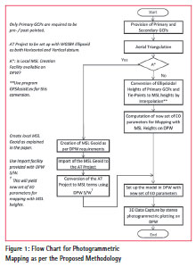
The flow chart for photogrammetric mapping as per the proposed methodology is given in Figure 1. We will now describe each step in detail in this section.
As can be seen from the flow chart, the proposed methodology with some modifications can also be employed without using the program GPSAssistLev, described in a separate section, in case the Digital Photogrammetric Workstation (DPW) software has the facility of creation of local MSL geoid with the help of a network of GCPs with known ellipsoidal and orthometric heights. Most of the modern DPWs do have this facility. The modified methodology is detailed in one of the following sections.
Provision of Ground Control Points (GCPs)
Provision of Primary GCPs
In the proposed solution, planimetric coordinates X, Y in UTM and height H (WGS84 Ellipsoidal height) of GCP’s are provided only at the corners of the photogrammetric block with the help of GPS. Such GCPs will be referred to as the Primary GCPs in this paper. The Primary GCPs will also include a few more GCPs to be provided in the photogrammetric block to serve as Check Points. No precision leveling of the Primary GCPs is required. However, all the Primary GCPs will need to be accurately transferred to the digital images. This does not pose much of a problem as the requirement of Primary GCPs is drastically reduced since this method makes full use of GPS/ IMU data.
Provision of Secondary GCPs
Uniformly distributed GCPs will be provided, 12 to 15 km apart, in the Area of Interest (AoI) by GPS with X, Y and H coordinates. These are referred to as Secondary GCPs in this paper. The Secondary GCPs will be connected to MSL height BMs by precision leveling to obtain their precise Orthometric Heights (h). Thus for each Secondary GCP, we will have both the Ellipsoidal Height (H) as a result of GPS survey and Orthometric Height (h) as a result of precision leveling.
Precise positioning of Primary Control Points on aerial imagery
In the methodology proposed, only the Primary GCPs, that would be very few in number due to reason explained earlier, need to be precisely positioned on the aerial photography. This can be best achieved by signalizing the GCPs on the ground prior to aerial photography (also known as pre-pointing) or by transferring the exact position of GCPs to the concerned aerial images, with the help of photos taken/ sketches made during GPS survey, after aerial photography (postpointing). Pre-pointing is more accurate but requires a lot of logistic support. There is no need of pre-pointing or post-pointing the Secondary GCPs in this method.
Aerial Triangulation (AT)
Based on the coordinates of Primary GCP’s so obtained (viz., X, Y in UTM and H as height above WGS ellipsoid), aerial triangulation is carried out to determine the precise tie-point coordinates in the same coordinate system as that of GCP’s. This is achieved by setting up the AT project in UTM coordinate system with WGS84 Ellipsoid as the Horizontal as well as the Vertical Datum. It may be noted that no Orthometric Heights are required for AT in the method proposed here. The AT will yield a large number of Tie-Points with X, Y and H coordinates whose Orthometric Height will not be known.
The AT will also yield six Exterior Orientation (EO) parameters for each image. These EO parameters can readily be used for generation of DTM in Ellipsoidal height system and precise orthophotos.
Conversion of Ellipsoidal Heights of the Primary GCPs and Tie- Points to Orthometric Heights
For each Secondary GCP, height of the MSL surface over the WGS84 ellipsoid is determined by subtracting the precision Leveling Height (h) from the corresponding Ellipsoidal Height (H) of the GCP. The Orthometric Height of all the Primary GCPs/ Tie-Points in the AoI is now computed as explained hereunder as per the mathematical model described in the next section.
(a) For each Primary GCP/ Tie-Point, the six parameters of 2nd order polynomial are computed by Least Squares solution of the equations, represented by equation (1) given in the next section, using the height differences (z) along with the X, Y values of at-least nine Secondary GCPs, that are nearest to the Primary GCP/ Tie-Point and the corresponding weight matrix. These nine Secondary GCPs are required, evenly spaced, in a 3×3 grid pattern for best results.
(b) The height of the MSL surface over the ellipsoid (z) at the Tie-Point/ Primary GCP location is then determined by equation (1) using the six parameters of the 2nd order polynomial and X, Y values of the point.
(c) Finally, the Orthometric Height is calculated by subtracting the z value from the ellipsoidal height of the point.
Computation of new set of EO Parameters for Mapping with Orthometric Heights
If the photogrammetric projects require the vector data/ DTM also as deliverables, such outputs are invariably required with heights above MSL. As such, the EO parameters, obtained by AT as described above, cannot be used for photogrammetric model set-up for generation of vector data/ DTM in MSL height system.
In the proposed method, therefore, a fresh set of EO parameters are determined by setting up the stereo models in a DPW by importing the AT measurements. All DPWs have this Import module that requires the adjusted image coordinates (x, y) and the terrain coordinates (X, Y, h), where h is the height above MSL, of all the points measured during AT (Primary GCPs and Tie-Points in this case) as input. This setup yields a new set of EO parameters which are then used for data capture for 3D vector mapping and DTM generation with heights in MSL system.
Mathematical model
A local MSL surface, represented by the six parameters of the following 2nd order polynomial, is modeled for each point whose height is to be determined by interpolation:
z = a0 + a1X + a2Y + a3XY + a4X2 + a5Y2 (1)
where,
z = H – h;
H = Ellipsoidal height of the GCP (measured by GPS)
h = Orthometric Height of the GCP (measured by precision field leveling)
X, Y are the UTM coordinates of GCP; and a0 to a5 are the six parameters of the 2nd order polynomial.
All the Secondary GCPs, falling within a specified Search Radius from the point with unknown Orthometric Height, are used as control points for generating the local MSL surface. Each such Secondary GCP yields one observation equation like (1). As already stated earlier, the Search Radius should be such that a minimum of nine control points (in a 3×3 pattern) are available for interpolation. For this, it is essential that Secondary GCPs with GPS coordinates (X, Y and H) and Orthometric Height (h) are provided in an approximate grid pattern (equally spaced at a certain interval), throughout the AoI. The optimal value of the interval depends on the required accuracy of Orthometric Height derived by interpolation and will be discussed at a later stage in this paper.
If there are n number of control points within the Search Radius from the point with unknown Orthometric Height, there will be n observation equations. These equations are solved by the method of Least Squares to yield the six parameters of the 2nd order polynomial. A weight equal to the inverse of the square of the distance of the control point from the point with unknown Orthometric Height is assigned to each observation equation. Together, these weights form the weight matrix that is used in the Least Squares solution of the observation equations. The weight matrix is a diagonal nxn matrix with the weights of the observation equations as diagonal elements.
A detailed treatment of the mathematical model, weight matrix and the Least Squares solution can be found in (Naithani, 1991).
Development of Computer Program GPSAssistLev
A computer program named GPSAssistLev has been developed in Microsoft Visual Studio C#.NET for GPS assisted densification of a leveling network, as per the algorithm based on the mathematical model outlined above. One of the inputs required by the program is the file containing the X, Y, H and h (both Ellipsoidal and MSL Heights) of the height control points (Secondary GCPs) and X, Y, H (only Ellipsoidal Height) of the points with unknown Orthometric Height, in this case the Primary GCPs and the Tie-Points. First, all the Secondary GCPs are entered in the file ending with ‘-99’ followed by all the Primary GCPs and the Tie-Points. The other input is the Search Radius which enables the program to short-list all the Secondary GCPs, which fall within this radius, for use in interpolation. The output of the program is a list of X, Y and h (orthometric height) coordinates with Point ID for all the Primary GCPs and Tie-Points contained in the input file.
Validity of Concept
The proposed methodology is based on the fundamental concept that the MSL surface is a smooth surface, of course with hills and valleys, but of very large wave lengths especially for the areas that are not highly mountainous. Even in highly mountainous terrain, the wave length of undulation remains significantly large making it amenable to derive precise Orthometric Heights by interpolation from a sparse precision leveling network without employing any gravimetric observations.
The smoothness of the WGS84 Geoid can be easily understood from the wellknown fact that despite the presence of mountains as high as 8,000 m (viz., Mt. Everest) and oceans as deep as 10,000 m (viz., Pacific Ocean), the separation between the WGS84 Geoidal surface and the WGS84 Ellipsoidal surface varies within a very small range, i.e., between +100 m to -100 m throughout the globe. Since an MSL surface is very nearly an equipotential surface, the smoothness of the MSL surface will be similar to that of a geoid. This is further confirmed by the results of Test Area A and Test Area B later elaborated in this paper.
Validation of Concept
Test data
To prove the concept and to determine the optimal spacing at which the Secondary GCPs with precise Orthometric Heights are required for the sparse leveling network, it was required to have some reliable test data. As we are well aware, it is a cumbersome process to obtain the Orthometric Heights in India and many other countries due to security concerns. Many countries, including US and Canada, provide facilities for conversion between Ellipsoidal Heights and Orthometric Heights for their respective territories.
In view of above, two test areas, Area A and Area B described hereunder, falling in Canadian territory, were selected to validate the concept. Each of these test areas measures 10 Latitude by 20 Longitude that translate to near rectangular areas each measuring approximately 100 km in North- South and 115 km in East-West direction.
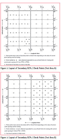
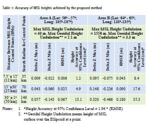
The test areas have been chosen pertaining to Canadian (and not Indian) territory only because of the availability of authentic data dealing with Ellipsoidal and Orthometric Heights. Natural Resources Canada (NRCan) provides the facility, online, for conversion from Ellipsoidal Heights to CGVD28 heights, (CSRS-A). The CGVD28 heights can very well be compared with the MSL Heights, (Hlasny, 2013). Using this online facility, the height of the MSL surface over the ellipsoid (H – h) was determined at every 7.5’ Lat x 15.0’ Longitude (thus, a total of 81 points for each test area). The heights of another set of 24 points for Test Area A and 30 points for Test Area B were also obtained in between the first set of points. The layouts of Secondary GCPs/ Check Points for Test Area A and B are given in Figure 2 and 3, respectively. The X, Y coordinates of all these points were also obtained in UTM coordinate system using another online facility, (CSRS-B).
(a) Test Area A: The area is bound by 560 N and 570 N Latitude and 1050 W and 1070 W Longitude. This terrain is undulating with terrain heights varying by 610 m (from 900 m to 290 m). The height of MSL surface above the Ellipsoid varies by 2.1 m (from -30.7 m to -28.6 m). The maximum separation of -30.7 m is at point with the height of 429 m and the minimum at the point with height of 888 m.
(b) Test Area B: The area lies between 640 N and 650 N Latitude and 1330 W and 1350 W Longitude. This area is quite hilly with terrain heights varying by 1,556 m (from 1,943 m to 387 m). The MSL separation from the ellipsoid varies by 3.3 m (from 8.6 to 5.3 m): the maximum at the point with height of 1,620 m and the minimum at the point with height of 657 m.
It may be seen that for both test areas, the maximum and minimum heights of MSL surface from the ellipsoid are not at the highest and the lowest terrain points.
Test Result and Analysis
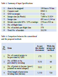
The accuracy of height achieved by this method is outlined in Table 1. It can be seen that the accuracy is dependent on the density and distribution of Secondary GCPs in the AoI.
For test area A pertaining to flat terrain, the height accuracy achieved is 1.2 cm, 4.9 cm and 13.1 cm for heights interpolated from Secondary GCPs provided at every 7.5’x15’ (12 km), 15’x30’ (25 km) and 30’x10 (50 km), respectively.
For test area B pertaining to hilly terrain, the accuracy achieved is 8.4 cm, 17.6 cm and 35.3 cm for heights interpolated from Secondary GCPs provided at every 7.5’x15’ (12 km), 15’x30’ (25 km) and 30’x 10 (50 km), respectively. From the above results, it can be categorically stated that if Secondary GCPs are available at every 12 km or so, the heights of points derived by the proposed method is suitable for contouring at a height interval of 25 cm. This will meet the requirements of most of the projects. For contouring requirement at 50 cm and 1 m interval, the spacing between Secondary GCPs could be as large as 25 km and 50 km, respectively. For less undulating terrain, the height accuracy would be suitable for even lower contour intervals.
However, particular care must be taken to get accurate GPS (ellipsoidal) heights on which the proposed method is based.
Application of the Proposed Method employing existing DPW software
From the above, it is well established that densification of leveling network employing the proposed method can be adopted for most of the photogrammetric mapping projects. The method may also be adopted employing any DPW system available in the market that allows creation of local geoid. The method of accomplishing this employing Socet Set DPW software is outlined in this section. The choice of Socet Set has been made only as an example. Any other DPW software with this facility can also be used.
Steps Involved
(a) Create AT project:
Create AT Project with the following datum:
– Horizontal datum: UTM/ WGS84 Ellipsoid
– Vertical datum: WGS84 Ellipsoid
The coordinates of the control points included for AT calculations will be in the above horizontal and vertical datum. The Primary GCPs established as per the earlier section will be used for this purpose. The Primary GCPs are required only at the corners of the photogrammetric block and will be very few in number. All these GCPs are required to be signalized prior to aerial photography or accurately positioned on images post aerial photography. Orthometric height of these GCPs is not required as input for AT.
(b) Aerial Triangulation:
Perform AT that includes automatic tie-point generation, GCP measurements, editing of tie-points, etc., and carry out AT adjustment employing suitable photogrammetric adjustment program as per the usual procedure.
(c) Create MSL geoid for the AT Project:
i. Derive the height of MSL surface over WGS 84 Ellipsoid (z) at all the Secondary GCP locations using the formula: z = Ellipsoidal Height – Orthometric Height.
ii. Prepare input ASCII file (in the format: X,Y, z) with values of X and Y coordinates in UTM and z value for all the Secondary GCPs provided throughout the AoI at a spacing of 12-15 km. It may be noted that signalization on ground or transfer of these GCPs on images is not required.
iii. The ASCII file so obtained will be imported into the AT project using DTM ASCII import of Socet Set. This will result in creation of MSL surface (or MSL geoid) for the AT Project.
(d) Convert the above AT project to MSL Project:
This is done employing the Create/ Edit utility of Socet Set (using MSL geoid created above) and saving it as an MSL Project. This will also yield the new Tie-Point and EO files with heights above MSL datum.
(e) Use of MSL project for Production:
Use the Converted AT Project for DTM/Ortho/3D Vector Data Generation or any other requirement. The height datum of DTM/Vector data so generated would be in MSL terms as is required by most clients.
Saving in overall cost and effort due to the proposed methodology
On the face of it, the time, effort and cost advantage resulting due to the proposed method may not appear significant due to the fact that leveling is still required. But if one works out the leveling effort required using the proposed method vis-àvis the leveling effort required otherwise, the advantage becomes very significant. There are other advantages too. A few GCPs need to be transferred to images that save a considerable effort. It also results in more automated aerial triangulation. In fact, this paper was triggered by the technical specifications of a tender by the Government of India for one of their major large scale mapping project, namely, the Integrated Coastal Zone Management Project, (SICOM, 2011). The tender pertained to aerial triangulation (AT) followed by production of DTM/Orthophoto/3D Vector data along coastal area of India employing DMC-1 aerial images acquired with air-borne GPS/IMU at 1:7,500 scale with fore and side overlaps of 60% and 25%, respectively. Full control points were required to be provided by relative static GPS observations and field levelingwhereas bands of height control points (BMs) were required to be provided by field leveling four models apart.
These specifications resulted in a very large number of plan control points and BMs increasing the cost of the project considerably, despite the fact that the imagery was acquired with onboard GPS/ IMU. To illustrate this point, we will now discuss the control requirement for a photogrammetric block of 100 km x 50 km as per the tender specifications and also as per the proposed methodology. For this discussion, we will assume the same input specifications as given in the tender document which are summarized in Table 2.
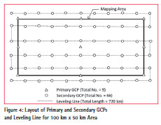
The total requirement and layout of Primary and Secondary GCPs and field leveling for photogrammetric mapping of the 100 km x 50 km block as per the methodology proposed in this paper is given in Figure 4. It may be noted from the figure that some Secondary GCPs are also provided a little outside the AoI to ensure the availability of a minimum of nine control points in a 3×3 pattern for the Primary GCPs and Tie-Points located at the periphery.
Comparison between the conventional and the proposed methods
The effort involved in provision of ground control points by GPS observations/ field leveling and pre-/post-pointing on aerial imagery for the two methods is summarized in Table 3. It can be seen that by adopting the proposed method, the number of GCPs to be provided by GPS reduces by 56%, the number of BMs to be provided by leveling reduces by 98%, the total length of leveling line reduces by 87%, and the number of points to be precisely pre- or post-pointed on aerial imagery by more than 99%. All this saving would have made the project much more economical and viable.
Conclusions
Photogrammetry is a very efficient and economical method of 3D mapping in advanced countries like US and Canada. GPS has become the de facto standard for provision of GCPs. The heights are still required in MSL terms, whereas GPS provides heights in Ellipsoidal terms. But it does not pose any problem since these countries have a precise geoid and a correction surface to automatically convert the GPS ellipsoidal heights to MSL terms.
However, this is not the case with countries like India that have not yet established their own geoid and correction surface. So these countries cannot make full use of airborne GPS/IMU though they have already acquired these technologies. As a result, these countries still insist on the conventional requirement of plan and height control for photogrammetry making the mapping projects quite uneconomical and unviable. So there is an urgent need for establishing a precise geoid and a correction surface for conversion of Ellipsoidal Heights to Orthometric Heights.
The establishment of precise geoid does require a lot of resources, planning and time. So till the time these countries are able to establish their own geoid, the method proposed in this paper provides an interim solution that makes full use of airborne GPS/IMU making mapping projects economical and viable.
Acknowledgements
I am grateful to Survey of India, where I have been closely associated with the R&D and digital mapping departments, and where I dealt with horizontal and vertical datum and also developed a module for generation of DEM from contours which has been taken further in this paper. I am equally grateful to COWI India Pvt. Ltd., to which I have been providing technical consultancy services in mapping and GIS during the last 8 years that also enabled me to understand the current mapping practices in US, Canada, Europe and other countries that have already established their own precise geoid and have facilities for conversion from GPS Ellipsoidal Heights to Orthometric Heights.
References
Canadian Spatial Reference System (CSRS-A) GPS·H 2.1 Geoid Height Transformation Program, URL: http:// www.geod.nrcan.gc.ca/apps/gpsh/gpsh_e. php (last date accessed: 21 May 2013).
Canadian Spatial Reference System (CSRS-B) Geographic to Universal Transverse Mercator (UTM), URL: http:// www.geod.nrcan.gc.ca/apps/gsrug/geo_e. php (last date accessed: 21 May 2013). Hlasny B., 2013.
The Canadian Height Modernization Initiative. Information for British Columbia Stakeholders / Clients, URL: http://archive.ilmb. gov.bc.ca/crgb/gsr/documents/ Attachment-InformationPaper- VerticalModernization.pdf (last date accessed: 31 August 2013): pp 1.
Milbert, Dennis G. and Smith, Dru A., 1996. Converting GPS Height into NAVD88 Elevation with the GEOID96 Geoid Height Model. A National Geodetic Survey, NOAA publication, URL: http:// www.ngs.noaa.gov/PUBS_LIB/gislis96. html (last date accessed: 31 August 2013).
NGS Geodetic Tool Kit. Online interactive computation of geodetic values. URL: http://www.ngs.noaa.gov/TOOLS/ (last date accessed: 31 August 2013). Naithani, K.K., 1991. DEM generation for the SOI PC / AutoCAD. ITC Journal 1991-2: pp 79-80.
SICOM, 2011. Bid Document for Provision of Ground Controls and Digital Photogrammetry. IFB No. Proc/SICOM/SOI/2011/01 Dated: 19/10/2011. URL: http://www.sicommoef. in/Data/Sites/1/docs/bid.pdf (last date accessed: 31 August 2013): pp 78.
Reproduced with permission from the American Society for Photogrammetry & Remote Sensing, Bethesda, Maryland, www.asprs.org


 (3 votes, average: 1.33 out of 5)


Leave your response!