VLBI geodetic precision with different models

Erhu WEI, Jingnan LIU, Peijing PAN

Very Long Baseline Interferometry (VLBI) is the unique space geodetic technique which can provide the Celestial Reference Frame (CRF), the Terrestrial Reference Frame (TRF) and the relationship between the two frames — Earth Orientation Parameters (EOP) at the same time. VLBI has a widely usage in space geodetic, ground geodetic, geophysical fields and so on. Presently, it can determine the position of the radio source outside the galaxy with 1mas precision, and determine several kilometers length of baseline on the earth’s surface with 1cm precision. Due to its high stability and high precision character, the Celestial Reference Frame outside the galaxy based on VLBI has been the best realization of the quasi-inertial referenceframe since 1980s. VLBI stations are the most important benchmarks in the International Terrestrial Reference Frame (ITRF), and VLBI is one main supporting technique which determines EOP. Till now, space and ground VLBI have accumulated more than 20 years’ data. They provide continuous and long-term data guarantee for space geodetic, ground geodetic and geographical research.

Though there are several kinds of common ocean tide and nutation models, there have no article giving us the best model combination through special comparison and analysis. This paper firstly introduces several common ocean tide models and nutation models, and then computes the global VLBI data during 2001-2007 using the OCCAM 5.0 software platform. It compares and analyzes the precision of geodetic parameter’s result using these models, and gives us the best ocean tide and nutation model combination.

Model introduction

OCCAM is a common software in processing space VLBI and ground VLBI data. It is used in describing the physical model of time delay and time delay rate, computing and adjusting all parameters’ partial derivative. Generally speaking, there are three physical models in this software[1]: 1) Computing model and setting up Standard Data File (SDF) model: the preparation of the data (DTAU0), precession and nutation and (PN), the correction of station’s displacement and partial derivative (STATION), geometry model (GEOMET), all five parts.
2) Adjusting scheme model: Kalman filter method, Least square method and least square collocate method, all three parts. 3) Application program model: obtaining information from the standard data files (SDF) in OCCAM, obtaining information from Obs-Calc files, all two parts.

OCCAM 5.0 software is made up of several executing programs. Only operating in definite sequence, we can get the accurate VLBI computing results. In this paper, we will compute with multi-baseline Kalman filter method, the detailed processing please refers to [2].

EANES model (CSR4.0 ocean loading model)

The EANES model[3] used in this paper is the CSR 4.0 ocean tide model, which is computed on the basis of the Orthotide model of Eanes et al., Center of Space Research, University of Austin, Texas, kindly made available to the world in April 1999. It is a further development of CSR 3.0 and contains 239 circles (about 6.4 years) of TOPEX/POSEIDON altimetry. Like the CSR3.0 ocean tide model, CSR4.0’s grid resolution is 0.5º×0.5º. It has the same orthotide frequency model; and it comprises the diurnal and semidiurnal bands.

For the computation of the loading effects, a land-ocean mask was constructed from ETOPO5. The same mask was used in CSR3.0. The reason for this is that many coastal model nodes of CSR3.0 inundate ETOPO5 land. Since the altimetry solution does not impose local water mass continuity conditions, the masking does not degrade global mass conservation (which is a more important error source in loading effects than in the tide elevation itself), but improves the realism of the load distribution. This model still uses concentrated load circling method and computes the close load through gradual reduction discrete points in the integral.

RAY model (GOT99.2b ocean loading model)

RAY Ocean tide model[4] is a long wavelength adjustment of FES94.1 using TOPEX/POSEIDON data and is given on a 0.5 by 0.5 degree grid.
FES94.1 Ocean tide model is a pure hydrodynamic tide model tuned to fit tide gauges globally. It has been calculated on a finite element grid with very fine resolution near the coast but the version used here is given on a 0.5 by 0.5 degree grid. GOT99.2b also becomes equal to FES94.1 outside the 66 degree latitudes.

Erhu WEI, Jingnan LIU, Peijing PAN

IAU 1980 nutation model

In 1979, J.Wahr and H.Kinoshita introduced re-comprehensive calculation for a practical nutation of the earth, they considered the force generated from earth’s solid tide to earth itself — deformation, nutation and rotation rate changes, and at the same time, they
thought about the natural effect and ellipse sphere delaminating effect in the matter of three main layers of the earth. They drew a conclusion in 1980, we call it “IAU 1980 nutation theory”[5].

HERING nutation model

The HERRING nutation model[1] in this software will compute the complete KSV_1996_3 nutation series with the associated corrections for planetary nutation, the freely excited Free- Core-Nutation (FCN), the precession constant change and a rate of change of obliquity. This model is designed from several aspects as following:

1) The Souchay and Kinoshita Rigid Earth KSRE95 nutation series;
2) Factors of the Retrograde FreeCore Nutation (RFCN) resonance factors from the nutation formula the Mathews et al.
3) The effects of annual modulation of geodetic precession;
4) A prograde annual nutation has been estimated along with the resonance coefficients;
5) The free RFCN mode was estimated once every two years for the data after 1984;
6) The new Simons et al., fundamental arguments are used in this version.

MHB_2000 nutation model

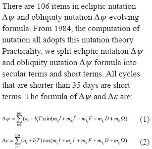
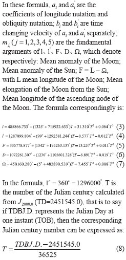
VLBI and LLR observations[6] showed that there are obvious defect existing in the IAU 1976 precession model and IAU 1980 nutation theory which have been the criterion for a long time. For example, these theoretical model doesn’t include the changing rate of obliquity in nutation that can’t be observed; the precession rate exists the difference about -3.0mas/yr between observation value and adoption value (the adoption value is too high); for nutation, the difference between observation model and adoption model exists about 20mas between each top. In short, the difference between the observations and models used in the past has exceeded the achieved observation precision far more. We need to get the nutation theory with including ocean tide’s and atmosphere’s non-rigid body and all in the order of magnitude of 0.1mas level known effect, and get the nutation series reaching the level of 5mas new rigid body earth. Based on many years of research, IAU 2000 convention[7] decided that the newly IAU 2000A precession-nutation model, that is MHB_2000 model (up to the level of the accuracy of 0.2mas) and IAU 2000B precession-nutation model (up to the level of the accuracy of 1mas) will replace the IAU 1976 precession model and IAU 1980 nutation theory. Improved precession rate, obliquity nutation changing rate, as well as the Celestial pole offsets consistent with newly precessionnutation model on J2000.0 epoch will be given in IERS 2003 convention.

MHB_2000 model[8] was proposed by Mathews, and it was developedon the basis of setting the problem of linear dynamic equation for wobbly nutation. It uses the estimated value of 7 parameters in the theory, obtains one newly precession-nutation VLBI data sequence in the theory of least squares. This nutation sequence depends on rigid earth nutation sequence found by Souchay (1999). It explains the change of geodynamical ellipticity implied by the observing correction of equator lunar-solar precession by the multiplier of 1.000012249. The new model contains the deviation between reference frames, geodetic precession and geodetic nutation. The Free Core Nutation (FCN) can’t be strictly forecast, so this model doesn’t include it. New precession-nutation model avoids the artificial separation in precession and nutation, but the precession model and nutation model is used separately in the system based on the spring equinox.

Tidal fluctuations in water height and currents will induce retrograde diurnal variation of equatorial oceanic angular momentum (OAM), hence small perturbation on nutation at the level of 1mas and most important contributions come from water height variations[9]. Considering the influence of anelasticity covering effect, the ocean tidal effect, electromagnetism coupling effect, which produced from the liquid outer core and solid core and the nonlinearity item. The MHB_2000 nutation model improves the accuracy of IAU 1980 nutation theory.

Erhu WEI, Jingnan LIU, Peijing PAN

The method of experiment

The data resource
In this experiment, we use the software of OCCAM 5.0 and the data in 2001-2007[10] computing the corresponding geodetic parameters. Based on the needs of the software, we choose the data of moderate memory (about 1M) to facilitate rapid comparative analysis.

The method of model combination
In order to compare the use of different software models in the results between the levels of accuracy, we classify these models into 6 items:
I In the calculation of the daily and sub-daily change of Earth Orientation Parameters (EOP) from ocean tide term, we choose EANES model; in the calculation of the precession and nutation, we choose IAU1980 nutation model;
II In the calculation of the daily and sub-daily change of Earth Orientation Parameters (EOP) from ocean tide term, we choose EANES model; in the calculation of the precession and nutation, we choose HERRING nutation model;
III In the calculation of the daily and sub-daily change of Earth Orientation Parameters (EOP) from ocean tide term, we choose EANES model; in the calculation of the precession and nutation, we choose MHB_2000 nutation model;
IV In the calculation of the daily and sub-daily change of Earth Orientation Parameters (EOP) from ocean tide term, we choose RAY model; in the calculation of the precession and nutation, we choose IAU1980 nutation model;
V In the calculation of the daily and sub-daily change of Earth Orientation Parameters (EOP) from ocean tide term, we choose RAY model; in the calculation of the precession and nutation, we choose HERRING nutation model;
VI In the calculation of the daily and sub-daily change of Earth Orientation Parameters (EOP) from ocean tide term, we choose RAY model; in the calculation of the precession and nutation, we choose MHB_2000 nutation model;

The criteria of precision compare
In the work of surveying, the power of the observation is the relative numerical indicator which denotes its precision. It is used in weighing various observation of different precision for handling these observations. For one group of observation, if its sigma is smaller, then its power is larger; or if its sigma is larger, its power is smaller. In this paper, the constant “FACTOR” means the value of the limitation for editing the data, the OCCAM software then sets this “FACTOR” value in the control files “KVLBI.OPT” and “KVLBI_ IE.OPT”, it can compute the limitation of the observation delay value subtract the computation delay value. If the difference between observation delay value and computation delay value is bigger than the “FACTOR” multiplies the expectation of the sigma, that is to say the precision obtained from this observation is not good, in this case, we will reduce the power of this observation (explained with * in this paper). If the number of the observations being reduced is too much, then the usability of this observation is small. The data of CHI-SQ is one indicator of reflecting the precision with kalman filter method, if its value is close to 1, then the precision of this result is good.

The analyze of the experiment result

Based on the combination of the above models, we compute the data following the chronological order:

The compare result by adopting the data of 2001
In calculating the data of the year 2001, after the relevant solution, we choose the better data 010424XE.NGS on April 24 to explain the result. The specific calculating result please refer to table1 (I- VI represent various combination of different models, the figures shown in this table represent the value of CHI-SQ): Table 1 the processing result of 010424XE.NGS

In the data processing on April 24 2001, we can see that if we choose ALGOPARK and FORTLEZA as the reference station for adjustment, in addition to the fourth group, the effects of the others are not ideal. After removing the results of these two stations, we average the other four stations, and then we get the first group of average.

Erhu WEI, Jingnan LIU, Peijing PAN

Tidal fluctuations in water height and currents will induce retrograde diurnal variation of equatorial oceanic angular momentum (OAM), hence small perturbation on nutation at the level of 1mas and most important contributions come from water height variations[9]. Considering the influence of anelasticity covering effect, the ocean tidal effect, electromagnetism coupling effect, which produced from the liquid outer core and solid core and the nonlinearity item. The MHB_2000 nutation model improves the accuracy of IAU 1980 nutation theory.

The method of experiment

The data resource
In this experiment, we use the software of OCCAM 5.0 and the data in 2001-2007[10] computing the corresponding geodetic parameters. Based on the needs of the software, we choose the data of moderate memory (about 1M) to facilitate rapid comparative analysis.

The method of model combination
In order to compare the use of different software models in the results between the levels of accuracy, we classify these models into 6 items:
I In the calculation of the daily and sub-daily change of Earth Orientation Parameters (EOP) from ocean tide term, we choose EANES model; in the calculation of the precession and nutation, we
choose IAU1980 nutation model;
II In the calculation of the daily and sub-daily change of Earth Orientation Parameters (EOP) from ocean tide term, we choose EANES model; in the calculation of the precession and nutation, we
choose HERRING nutation model;
III In the calculation of the daily and sub-daily change of Earth Orientation Parameters (EOP) from ocean tide term, we choose EANES model; in the calculation of the precession and nutation, we choose MHB_2000 nutation model;
IV In the calculation of the daily and sub-daily change of Earth Orientation Parameters (EOP) from ocean tide term, we choose RAY model; in the calculation of the precession and nutation, we choose IAU1980 nutation model;
V In the calculation of the daily and sub-daily change of Earth Orientation Parameters (EOP) from ocean tide term, we choose RAY model; in the calculation of the precession and nutation, we choose HERRING nutation model;
VI In the calculation of the daily and sub-daily change of Earth Orientation Parameters (EOP) from ocean tide term, we choose RAY model; in the calculation of the precession and nutation, we choose MHB_2000 nutation model;

The criteria of precision compare
In the work of surveying, the power of the observation is the relative numerical indicator which denotes its precision. It is used in weighing various observation of different precision for handling these observations. For one group of observation, if its sigma is smaller, then its power is larger; or if its sigma is larger, its power is smaller. In thispaper, the constant “FACTOR” means the value of the limitation for editing the data, the OCCAM software then sets this “FACTOR” value in the control files “KVLBI.OPT” and “KVLBI_ IE.OPT”, it can compute the limitation of the observation delay value subtract the computation delay value. If the difference between observation delay value and computation delay value is bigger than the “FACTOR” multiplies the expectation of the sigma, that is to say the precision obtained from this observation is not good, in this case, we will reduce the power of this observation (explained with * in this paper). If the number of the observations being reduced is too much, then the usability of this observation is small. The data of CHI-SQ is one indicator of reflecting the precision with kalman filter method, if its value is close to 1, then the precision of this result is good. The analyze of the experiment result Based on the combination of the above models, we compute the data following the chronological order: The compare result by adopting the data of 2001 In calculating the data of the year 2001,
after the relevant solution, we choose the better data 010424XE.NGS on April 24 to explain the result. The specific calculating result please refer to table1 (I- VI represent various combination of different models, the figures shown in this table represent the value of CHI-SQ): Table 1 the processing result of 010424XE.NGS In the data processing on April 24 2001, we can see that if we choose ALGOPARK and FORTLEZA as the reference station for adjustment, in addition to the fourth group, the effects of the others are not ideal. After removing the results of these two stations, we average the other four stations, and then we get the first group of average. 20 |

The analyze of the experiment result

Based on the combination of the above models, we compute the data following the chronological order:

The compare result by adopting the data of 2001
In calculating the data of the year 2001, after the relevant solution, we choose the better data 010424XE.NGS on April 24 to explain the result. The specific calculating result please refer to table1 (I- VI represent various combination of different models, the figures shown in this table represent the value of CHI-SQ): Table 1 the processing result of 010424XE.NGS.

In the data processing on April 24 2001, we can see that if we choose ALGOPARK and FORTLEZA as the reference station for adjustment, in addition to the fourth group, the effects of the others are not ideal. After removing the results of these two stations, we average the other four stations, and then we get the first group of average.

Table 1 the processing result of 010424XE.NGS

Table 2 the processing result of 020711XE.NGS

Table 3 the processing result of 031021XE.NGS

Table 4 the processing result of 040601XA.NGS

Erhu WEI, Jingnan LIU, Peijing PAN

Table 5 the processing result of 2005.08.25, 2006.09.21 and 2007.10.21

Table 6 the general result of all kinds of combination

The compare result by adopting the data of 2002
In calculating the data of the year 2002, after the relevant solution, we choose the better data 020711XE.NGS on July 11 to explain the result, the specific calculating result please refer to table2 (I – VI represent various combination of different models, the figures shown in this table represent the value of CHI-SQ):

In the data processing on July 11 2002, we can see that if we choose FORTLEZA and ALGOPARK as the reference station for adjustment, in addition to the first group, the effects of the others are not ideal. When choosing MATERA as the reference station to calculate, all six groups’ precision are not ideal. After removing the results of these three stations, we average the other three stations, and then we get the second group of average.

The compare result by adopting the data of 2003
When we processed the data on October 21 2003, we found that there were a considerable number of observations were reduced their power, and their availability and the results is not very good to deal with. In the final model comparison, we choose not to consider this data. The specific calculating result please refer to table3 (I – VI represent various combination of different models, the figures shown in this table represent the value of CHI-SQ):

The compare result by adopting the data of 2004
In calculating the data of 2004, after the relevant solution, we choose the better data 040601XA.NGS on June 1 to explain the result, the specific calculating result please refer to table4 (I – VI represent various combination of different models, the figures shown in this
table represent the value of CHI-SQ):

In the data processing on June 1 2004, we can see that if we choose TIGOCONC and WESTFORD as the reference station for adjustment, in addition to the

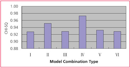
Figure 1 the general result of all kinds of combination

second and sixth group, the effects of the others are not ideal. After removing the results of these two stations, we average the other three stations, and then we get the third group of average.

The result by adopting the data of 2005-2007
Adopting this method, we get the results on August 25 2005, September 21 2006, October 21 2007, the final processing result please refer to table 5 (I – VI represent various combination of different models, the figures shown in this table represent the value of CHI-SQ):

Compared results
After doing these works, we compute the precision of various model combinations, and list the result with table 6: (I – VI represent various combination of different models, the figures in this table represent the value of CHI-SQ): Then we represent the result correspondingly create the figure 1:

From figure 1 and table 6, we can see that in these six kinds of categories, the fourth model of the results of the final classification sought by the CHISQ value is 0.9728, the closest to 1.00. Though the precision of the other combinations is near 1.00 too, their gap is very small. We believe that in the same circumstance, choosing the combination of RAY ocean tide model and IAU_1980 nutation model is the best choice.

Conclusion
On the basis of briefly introducing several common ocean tide models and nutation models, this paper uses the OCCAM 5.0 software platform and the global VLBI data during 2001-2007, compares and analyzes the precision of the geodetic parameter result getting from these models. The final results show that: using RAY ocean tide model and IAU_1980 nutation model, we can obtain the best precision result in this kind of model combination. This paper has done basic work for future data processing and analyzing.

Acknowledgement

This research is funded by the national ‘973 Project’ of China (No 2006CB701301), the national ‘863 Project’ of China (No. 2008AA12Z308) the National Natural Science Foundation of China(No. 40774007), and the project of university education and research of Hubei province (No. 20053039).

Reference

1] O.Titov, V.Tesmer, J.Bohem. OCCAM 5.0 USER’S GUIDE
2] Erhu Wei, Jingnan Liu, Zhenghang Li, Chuang Shi. The simulated computation of estimating geodetic parameters with space VLBI observations. Journal of Wuhan university science edition, 2006,31(10): 875~878
3] ftp://gere.oso.chalmers.se/pub/ hgs/oload/#olcs41.readme#
4] http://www.oso.chalmers. se/%7Eloading/tidemodels.html
5] Zhenghang Li, Debao Xu, Yiying Dong, Caizhang liu. The fundament of space geodetic theory. Wuhan: Mapping Wuhan University of Science and Technology Publishing House,1998
6] Liande Pan. The newly reference system in criterion and the related issues. Shanxi observatory Journal. 2002[25]: 131~140
7] IAU Information Bulletin 88.Resolution B1.6.2001
8] O.Titov, V.Tesmer, J.Bohem. OCCAM 6.2 USER’S GUIDE
9] http://hpiers.obspm.fr/eop-pc/ models/nutations/nut_oceanic.html
10] http://mars.hg.tuwien. ac.at/~vlbi/db2/