
| Geodesy | |
Local Moho estimation using gravity inversion
Gravity inversion is a useful tool for determining Moho depths in regions without having adequate seismic information |
 |
|
Composite of the Earth’s Crust and Moho Estimation
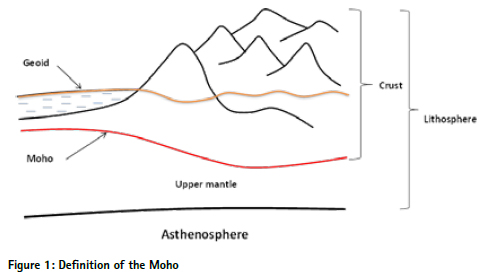
Generally, the Earth is comprised three main internal structures: crust, mantle and core. These structures have different densities and seated in different depths. The innermost part of the Earth is the core and has the highest density. The solid inner core, which mainly consists of iron with a small amount of nickel, is surrounded by a liquid outer core and together with this outer core creates Earth’s magnetism (Lowrie, 2007). The outermost part, the crust, covers the mantle which is located in between the core and crust and divided as upper and lower parts. Although the composition of solid lower mantle is poorly known, it is supposed to consist of magnesium and oxides of iron (Lowrie, 2007) and covered by plastic upper mantle. The crust together with the top layer of mantle, which is partially malted and bounded by the asthenosphere, is called the lithosphere and can be divided into seven or eight large pieces (or plates): African, Antarctic, Eurasian, North American, South American, Pacific and Indo-Australian (Indian and Australian), and dozens of smaller plates (http://en.wikipedia.org/wiki/Plate_ tectonics). Even though the crust contains very less volume of the Earth (less than 1%), the discovery of crust’s properties is extremely important from a geological point of view since it is the place where all our geological resources like natural gas, oil and minerals come from.
The boundary between the Earth’s crust and mantle is termed the Mohorovičić discontinuity, usually called Moho. A Croatian seismologist, named Andrija Mohorovičić first discovered this boundary in 1909. He noticed that seismograms from shallow-focus earthquakes had two sets of P (Primary) and S (Secondary) waves: one follows the direct path near the surface and the other refracted by the high density medium. He distinguished these two velocity mediums as lower and higher density interior layers where seismic waves acquire higher velocity in higher density medium. The lower density medium is now commonly referred to as Earth’s crust while the higher density medium below the crust is known as Earth’s mantle. The density interface between these two layers was named after him as Mohorovičić discontinuity (Moho). The realizing of Moho is vital from geological point of view because once the gravity effect of Moho structure is determined, it can be removed from observed gravity leaving the gravity effect of crustal structure which is important to identify the composite of the crust.
Moho estimation techniques
Generally, seismic and isostaticgravimetric methods are used to determine Moho. The seismic methods usually provide a realistic way of imaging crustmantle interface (Moho). However, the limited coverage of seismic data due to the cost and effort involved in collecting the data makes its application difficult for Moho estimation in some regions. An alternative could be the use of gravity data in isostatic-gravimetric methods. The main principle of isostatic methods which define topographic compensation masses is based on “equal-pressure and equal-mass” hypotheses. Two different methods have been developed at almost exactly the same time based on these hypotheses: Pratt-Hayforg system (1854) and Airy-Heiskanen system (1855). The former assumes varying crustal density with a uniform depth, termed as level of compensation. The latter supposes varying crustal thickness with uniform density, which forms roots and anti-roots. Both systems are highly idealized and assume the compensation to be local.
By introducing regional instead of local compensation, Vening Meinesz modified the Airy system in 1931 assuming that the crust is a homogeneous elastic plate floating on a viscous mantle (Bagherbandi and Sjöberg, 2012b) and later the system was further generalized and discussed by Moritz (1990) considering spherical effects. However, the homogeneity of plates is hardly believed since many geophysical evidences have proved that the density variations inside the plates and various non-isostatic effects introduce isostatic anomalies which violate the fundamental assumption of the inverse problem of isostasy (Sjӧberg, 2009). The isostatic-gravimetric methods of Moho estimation deal with this isostatic anomalies together with a suitable isostatic model and recently Vening Meinesz-Moritz isostatic model was used as it is the most realistic model among the traditional isostatic models. Isostatic anomalies can also be used as a classical-spectral approach of Moho estimation (Braitenberg et al., 2000).
The pure gravimetric method of Moho estimation is based on an inversion of the gravity data. Usually, Bouguer anomalies are used for the inversion. The advantage of gravity inversion is the accessibility of gravity data since the satellite gravity data together with the terrestrial data provides a sufficient coverage for the whole globe (Block et al., 2009). The global geopotential models are also an important source of gravity information (Reguzzoni and Sampietro, 2012). The most important role of gravity inversion method is to extract the appropriate anomalies related to Moho deflection. Many techniques have been employed to isolate anomalies associated with these Moho discontinuities (Lefort and Agarwal, 2000). Spectral methods are used to filter short and long wavelength effects of gravity stem from intracrustal/ superficial inhomogeneities and deep seated sources (Sjoberg, 2009). To decide which wavelengths should be filtered out or which range of wavelengths should be used is very difficult and complex. It usually depends on the target depth, spectrum analysis of the gravity anomaly, and other geophysical or geological information (Gomez-Ortiz et al., 2011).
The global Moho models
Seismic methods of Moho estimation are based on the changes of the velocity of the propagated seismic waves between the crust and mantle. CRUST5.1 is the first official global seismic crustal model published by Mooney et al. (1998). The resolution of this model is 5° x 5°. This model is updated to CRUST2.0 by Bassin et al. 2000 (resolution 2° x 2°) employing the seismic data published in the period 1984-1995. Now CRUST1.0 model is available with 1° x 1° resolution (https:// igppweb.ucsd.edu/~gabi/crust1.html). This model gives rather comprehensive density structure of the crust and upper mantle. The model comprises seven layers: ice, water, soft sediments, hard sediments, upper crust, middle crust and lower crust. The 7th layer (lower crust) represents the Moho depths with respect to MSL. Apart from the elevations of the different density layers, the model gives the density variation of each layer.
The first global high resolution (0.5° x 0.5°) map of Moho depths, GEMMA (GOCE Exploitation for Moho Modeling and Applications), was compiled based on data from ESA’s GOCE gravity satellite. This global model is computed by inverting the global grid of second radial derivative of the gravitational potential (gravity gradient) observed by GOCE satellite and considering the density of the crust as defined in the CRUST2.0 model. For the computation of this model, gridded satellite data have been combined with sparse ground data using collocation (Reguzzoni and Sampietro, 2012). GEMMA global and local models are available at http:// geomatica.como. polimi.it/elab/gemma/.
Even though global Moho models cover whole globe, their accuracies are not well specified. The accuracy of global seismic CRUST models depends on the data availability and is varies from place to place. For instance, the model gives more accurate Moho depths in United States and Europe since most of the seismological data are confined to these regions (see the distribution of global seismological data and network stations at http://www.isc.ac.uk/ and http://www.iris. edu/hq/programs/gsn). The accuracy of GEMMA model is also not consistent in continental and marine regions due to the variation of crust-mantle density contrast.
Gravity inversion
One of the fundamental challenges of geophysical study is to determine the geometry of subsurface structure (density interfaces) from gravity anomaly. One such an important application is to map crust-mantle boundary (Moho) from surface gravity anomaly. The solution of this problem can be categorized into two main modeling techniques: forward and inverse (Ebbing et al., 2001). In forward modeling method, the gravity effect is computed for an initial model source body constructed based on geological and geophysical intuition and then compared with the observed gravity anomaly. The final source body is developed by adjusting model parameters to fit the computed and observed anomalies.
In the inverse method, the parameters of the perturbing body are computed directly from the observed anomalies. This method becomes more popular after adopting FFT algorithms. Braitenberg et al. (1997) proposed an iterative method from isostatic gravity anomalies with an initial isostatic Moho. The other important FFT application in gravity forward modeling was presented by Parker (1973). He expressed the total gravitational anomaly due to uneven, non-uniform layer of material in terms of its Fourier transform by means of the sum of Fourier transforms of powers of the surface affecting the anomaly. The corresponding inverse scheme was presented by Oldenburg (1974). He rearranged Parker’s forward algorithm to determine the density interface from the observed gravity anomaly. Although the original form of Parker-Oldenburg’s algorithms is two-dimensional (2D), its three-dimensional (3D) application with large data sets in geophysical field can still be frequently found now (Gómez– Ortiz and Agarwal, 2005). The Parker- Oldenburg algorithms were used in this article for numerical analysis.
Usually high frequency filtered Bouguer gravity anomaly data is used for Moho depth estimation from gravity inversion. As mentioned earlier, the extraction of the most relevant gravity anomaly that reflects main Moho deflections is complex since the harmonics of the short wavelength features could be mixed with that of long wavelength features. To overcome this difficulty, various filtering techniques are used. Spectral methods are used to filter short and long wavelength effects of gravity that stem from intracrustal/ superficial inhomogeneities and deep seated sources (Sjöberg, 2009). However, to decide which wavelengths should be filtered out or which range of wavelengths should be used is very difficult and complex. It usually depends on the target depth, spectrum analysis of the gravity anomaly, and other geophysical or geological information.
Gravity data filtering and spectral analysis
Usually, the shallow gravity effects are due to intracrustal and superficial inhomogeneities (Bagherbandi et al., 2013). Although spectral window method (Spector and Grant, 1970) removes short wavelength effects of gravity data, some shallow features such as the sedimentary cover are broadband. This demonstrates that the effects of these shallow features cannot be removed completely by spectral filtering (Corchete et al., 2010). Therefore, the gravity effect of sedimentary layer should be removed first from Bouguer anomalies before starting spectral analysis (Sjöberg, 2009), otherwise the spectrum of features at shallow depths could overlap spectrum of deep features (as Moho undulations).
To obtain the gravity anomalies associated with the lithosphere structure, the gravity effect of features deeper than lithosphere and non-isostatic effects must be subtracted. The main long wavelength gravity effects are coming from density variation of Earth’s mantle and core/ mantle structure variations (Martinec, 1994). These deep mass anomalies and other various long wavelength gravity effects can be categorized as nonisostatic effects which correspond to the influence of different geophysical mechanisms such as crustal thickening/ thinning due to thermal expansion of mass of the mantle, mantle convection, plate movements and flexure (Watts, 2001). Generally, if the topography contains features longer than ~500 km, it may contain a component of the surface expression of mantle convection (Crosby, 2007). However, a proper analysis is needed since the depth of these source structures is location dependent. These deep gravity effects are estimated from the spectral depth of the gravity signal using the degree based on Bruns’ formula (Bagherbandi and Sjöberg, 2012a).
Numerical study
Numerical studies were carried out in a test region of USA, bounded by latitudes 30–43 N and longitudes 128–112W, where reasonably accurate seismic Moho depths were available for validation of the results. The Parker- Oldenburg algorithms were used for the computations (Prasanna et al, 2012).
A dataset of 1193 seismic Moho depths, which were compiled from numerous seismic observations and datasets of this area (Tape et al., 2012), was used for comparison of the results. According to this data, the average Moho of this area is about 26 km with minimum 6 km and maximum 53 km. The large variation of the Moho is the result of the transition from oceanic crust to continental crust. The average uncertainty of this published Moho was 2.3 km.
The gravity effect of sedimentary layer was removed based on CRUST2.0 model. For long wavelength correction, it was assumed that the mean crustal thickness would be less than 40 km (According to CRUST2.0 and the seismic data, the mean Moho depth of the area is 23 km and 26 km respectively). Therefore, the spectral depth up to 40 km, were excluded, based on spectral depth estimation, as being caused by non-isostatic effects. The remaining Bouguer anomalies were used for spectral analysis to find the appropriate frequency range related to Moho deflection. From spectral analysis we found that the wavelength range 157–95 km was most accountable for mean CRUST2.0 Moho depth.
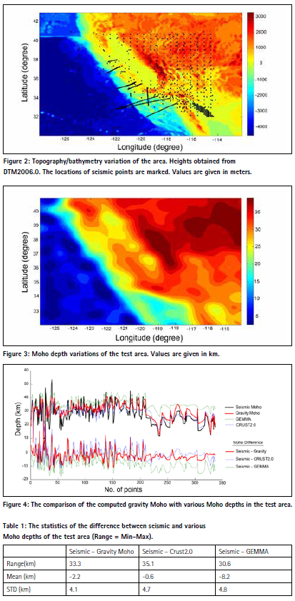
Finally, the high cut-off filter was used with the selected frequency range to determine the Moho surface (Figure 3) following the inversion process.
To validate the results of the test area, a part of the dataset (337 points) located well within the test area was selected from the available seismic database. Additional comparisons were made using CRUST2.0 and GEMMA global Moho depths. Figure 4 and Table 1 show the statistics of the comparison.
The comparison was carried out at three levels. First, the gravity Moho depths are compared with seismic Moho depths. This will give the actual deviation of the gravity Moho surface. Secondly, the difference with CRUST2.0 Moho will show how consistent the gravity Moho surface is with the best global seismic Moho model available so far. Finally, we will test our computed gravity Moho against a global gravity Moho model (GEMMA) compiled from different techniques.
Generally, our computed Moho depths are well-consistent with the seismic Moho depths (correlation coefficient is around 0.8). From Table 1, we could notice that all three different Moho depths have a similar standard deviation range (4–5 km standard deviation of the difference). However, the mean difference between our computed gravity Moho and the actual seismic Moho is significantly lower than that of GEMMA Moho. The possible reason of having a large bias in GEMMA Moho (8.2 km) would be that the density contrast of Moho interface used in GEMMA project is significantly different from the seismic Moho interface. The bias of our computed gravity Moho (2.2 km) could be due to using the mean value of density contrast (0.4 g/cm3). However, this bias may be acceptable since the average uncertainty of seismic Moho is 2.3 km (Tape et al., 2012). CRUST2.0 Moho is almost consistent with observed seismic Moho. This is expected, because the most of seismic points in this area are included in CRUST2.0 model. Finally, we could say that our computed Moho obtained is more or less the same quality (our model is slightly better) as Global Moho models, and most importantly our Model is better in terms of the resolution (5 arc min).
Conclusion
Moho depths were computed using an interactive way of gravity inversion method constrained with seismic information (CRUST2.0 data). The result of the test area demonstrated that it has better consistency with seismic Moho depths than global Moho depths in terms of resolution and accuracy, suggesting that this method is suitable for high resolution local Moho depth determination, especially for areas without adequate seismic data.
The determination of Moho surface is important in various geophysical studies, such as studies of crustal and lithosphere signature and flexure studies. Usually, geophysical/structural studies deal with large areas, for instance, continental or regional studies. However, the recovery of local Moho with high resolution is important for local geophysical studies, such as studies of density distribution of the crust and small-scale subduction
References
Bagherbandi, M. and Sjöberg, L. E. (2012a). Non-isostatic effects on crustal thickness: A study using CRUST2.0 in Fennoscandia. Physics of the Earth and Planetary Interiors, 200-201, 37-44.
Bagherbandi, M. and Sjöberg, L. E. (2012b). A synthetic Earth gravity model based on a topographicisostatic model. Studia Geophysica et Geodaetica, 56(4), 935-955.
Bagherbandi, M., Tenzer, R., Sjöberg, L. E. and Novák, P. (2013). Improved global crustal thickness modeling based on the VMM isostatic model and non-isostatic gravity correction. Journal of Geodynamics, 66, 25-37.
Bassin, C., Laske, G. and Masters, G. (2000), The current limits of resolution for surface wave tomography in North America, EOS Trans. AGU, 81(48), Fall Meet. Suppl., Abstract S12A-03.
Block, A. E., Bell, R. E. and Studinger, M. (2009). Antarctic crustal thickness from satellite gravity: Implications for the Transantarctic and Gamburtsev subglacial mountains. Earth and Planetary Science Letters, 288(1), 194-203.
Braitenberg, C., Pettenati, F. and Zadro, M. (1997). Spectral and classical methods in the evaluation of Moho undulations from gravity data: The NE Italian Alps and isostasy. Journal of Geodynamics, 23, 5-22.
Braitenberg, C., Zadro, M., Fang, J., Wang, Y. and Hsu, H. T. (2000). Gravity inversion in Qinghai-Tibet plateau. Phys. Chem. Earth, 25(4), 381-386.
Corchete, V., Chourak, M. and Khattach, D. (2010). A methodology for filtering and inversion of gravity data: An example of application to the determination of the Moho undulation in Morocco. Engineering, 2(3), 149-159.
Crosby, A. G. (2007). An assessment of the accuracy of admittance and coherence estimates using synthetic data. Geophysical Journal International, 171, 25-54.
Ebbing, J., Braitenberg, C. and Götze, H. J. (2001). Forward and inverse modelling of gravity revealing insight into crustal structures of the Eastern Alps. Tectonophysics, 337, 191-208.
Gómez-Ortiz, D. and Agarwal, B. N. P. (2005). 3DINVER.M: A MATLAB program to invert the gravity anomaly over a 3D horizontal density interface by parkeroldenburg’s algorithm. Computers & Geosciences, 31, 513-520.
Gómez-Ortiz, D., Agarwal, B. N. P., Tejero, R. and Ruiz, J. (2011). Crustal structure from gravity signature in the Iberian Peninsula. Geological Society of America Bulletin, 123(7-8), 1247-1257.
Lefort, J. P. and Agarwal, B. N. P. (2000). Gravity and geomorphological evidence for a large crustal bulge cutting across Brittany (France): A tectonic response to the closure of the Bay of Biscay. Tectonophysics, 323(3–4), 149-162.
Lowrie, W. (2007). Fundamentals of geophysics (Second edition), Cambridge University Press.
Martinec, Z. Ě. K. (1994). The minimum depth of compensation of topographic masses. Geophysical Journal International, 117(2), 545-554.
Moritz, H. (1990). The Figure of the Earth. H Wichmann, Karlsruhe. Oldenburg, D. W. (1974). The inversion and interpretation of gravity anomalies. Geophysics, 39(4), 526-536.
Parker, R. L. (1973). The rapid calculation of potential anomalies. Geophysical Journal of the Royal Astronomical Society, 31, 447-455.
Reguzzoni, M. and Sampietro, D. (2012). Moho estimation using GOCE data: A numerical simulation. In S. C. Kenyon, M. C. Pacino and U. J. Marti (Eds.), International Association of Geodesy symposia, “geodesy for planet earth”, Springer, Verlag, Berlin, 205-214.
Sjöberg, L. E. (2009). Solving Vening Meinesz-Moritz inverse problem in isostasy. Geophysical Journal International, 179(3), 1527-1536.
Spector, A. and Grant, F. S. (1970). Statistical methods for interpreting aeromagnetic data. Geophysics, 35, 293-302.
Watts, A. B. (. (2001). Isostasy and flexure of the lithosphere. Cambridge University Press, Cambridge, New York, Melbourne


 (No Ratings Yet)


Leave your response!