GNSS Constellation Specific Monthly Analysis Summary: August 2026

Oct 2026 | No Comment

The analysis performed in this report is solely the author’s work and his opinion.

Narayan Dhital

Actively involved to support international collaboration in GNSS related activities. He has regularly supported and contributed to different workshops of the International Committee on GNSS (ICG), and the United Nations Office for Outer Space Affairs (UNOOSA). As a professional employee, the author is working as GNSS expert at the Galileo Control Center, DLR GfR mbH, Germany

1. Introduction

This article continues the monthly performance analysis of the GNSS/SBAS constellation. Readers are encouraged to refer to previous issues for foundational discussions and earlier results. The focus for this month’s issue is the atomic time generation and GNSS synchronization. A sample data from BIPM learning platform is used to demonstrate how clock ensemble produces atomic time that can be the national laboratory time or the GNSS system time. It is solely for educational purposes.

1. Atomic timescale generation: A practical overview

The generation of a local atomic timescale, Temps Atomique (TA), lies at the heart of modern timekeeping and navigation. Laboratories worldwide maintain ensembles of atomic clocks—hydrogen masers and cesium standards—to realize their local timescale, UTC(k), which is then compared and steered toward Coordinated Universal Time (UTC). This ensemble approach ensures continuity and stability, as no single clock can provide perfect performance across all timescales. Applications of such timescales extend from GNSS synchronization and telecommunications to metrology, where nanosecond precision defines the accuracy of global systems. The ensemble average, computed through weighted clock data, forms the laboratory’s provisional timescale (UTC(k)-TA), which is later aligned with UTC through international comparisons coordinated by the BIPM.

2. Example Clock Ensemble

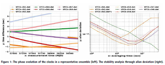
The initial plots of the raw clock data (Figure 1) illustrate the phase evolution of individual clocks relative to a chosen reference. Each curve represents a clock’s time difference over Modified Julian Date (MJD), revealing distinct frequency drifts—some clocks run slightly faster, others slower. The slopes of these lines correspond to frequency offsets, while their spread indicates the diversity of the ensemble. The accompanying Allan deviation plot characterizes each clock’s stability: maser-like clocks exhibit excellent short-term stability (low deviation at small averaging times), whereas cesium clocks dominate longterm stability (low deviation at large averaging times). In this ensemble, clk3 and clk8 behave as hydrogen masers with superior short-term precision, while clk4 and clk7 resemble cesium standards, offering long-term robustness. Clk2 shows a discontinuity and could impact the ensemble if not treated carefully. Together, these behaviors define the foundation for constructing a smooth, weighted atomic timescale.

3. Weighted TA Generation

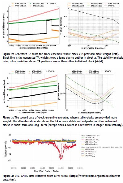
Two ensemble averaging cases demonstrate the impact of weighting. In the first case, random weights were assigned, including high weight to a discontinuous clock (clk2), resulting in a jump in the averaged timescale (Figure 2)—a clear sign of instability. The averaged curve failed to remain continuous, showing how improper weighting can distort the ensemble output. In the second case (Figure 3), weights were redistributed to favor the most stable clocks: higher weight for clk3 (maser-like short-term stability), moderate for clk4 and clk7 (cesiumlike long-term stability), and minimal for noisy clocks. By assigning higher weight to clk3 for shortterm precision, emphasizing clk4 for longterm robustness, and keeping moderate weights for clk5 and clk7, the ensemble average achieves a balance that suppresses noise while maintaining continuity. The resulting UTC(k)-TA curve became smoother and more stable, lying below most individual Allan deviation traces. This demonstrates how careful weighting suppresses noise and drift, producing a continuous and reliable timescale. However, the process must remain dynamic—weights should adapt as clock performance evolves to prevent discontinuities when clocks join or leave the ensemble.

4. GNSS-UTC Offset and Synchronization

Each GNSS constellation—GPS, Galileo, BeiDou, and GLONASS—maintains its own internal system time using the same ensemble principle. The control segment averages multiple atomic clocks, applying stability-based weights to generate GPS Time (GPST), Galileo System Time (GST), and BeiDou Time (BDT). These system times are continuously steered toward UTC using frequency adjustments derived from for example GNSS common-view comparisons, monitoring links coordinated by national laboratories/ BIPM. The GNSS–UTC offset plot (Figure 3) shows these relationships: most systems remain within a few nanoseconds of UTC, confirming precise steering. The exception, GLONASS, exhibits a temporary excursion around MJD ≈ 61200, likely due to a control-segment anomaly. The dotted curves represent the broadcast UTC corrections (bUTC) included in navigation messages, enabling receivers to convert system time to UTC in real time. Thus, the GNSS–UTC offsets are the operational link between constellation timescales and the global UTC framework— the same principle applied when steering a laboratory’s UTC(k)-TA toward UTC.

Note that UTC-GNSS constellation specific offset analysis was provided as monthly graph in the mycoordinates up until January 2026. Viewers are encouraged to go through them and also check BIPM web interface for latest data

5. Conclusions

The ensemble averaging process is fundamental to atomic timescale generation and a diverse set of clocks generate more robuts and reliable time. But it is not without challenges. Weighted TA computation can become problematic when clocks exhibit discontinuities or when members of the ensemble are replaced, causing abrupt changes in the averaged output. Such events can introduce phase jumps or distortions that compromise continuity. To mitigate this, laboratories employ prediction-based approaches, where the timescale is extrapolated using past stability data and frequency trends rather than instantaneous averaging. This predictive steering ensures smoother transitions and resilience against clock changes. The next article will explore this prediction method, detailing how it enhances the robustness of UTC(k) generation and supports global synchronization across GNSS and metrology networks.