Mitigating the systematic errors of e-GPS leveling

Lao-Sheng Lin Associate Professor, Department of Land Economics National Chengchi University, Taiwan

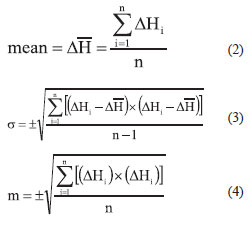
e-GPS (Electronic Global Positioning System), used in Taiwan, is a kind of real-time kinematic satellite positioning technology as VRS-RTK (Virtual Reference Station Real Time Kinematic).

Because of basing on different vertical datum, any point on the surface of the Earth, its ellipsoidal height h and orthometric height H are different. The height difference between h and H is called undulation N. Suppose it can be ignored that the vertical deflection on ground is very small, then any point on the ground, the relationship among h, H and N, can be represented it with a simple mathematical equation: h = H+N(Hu, et al., 2004; Kavzoglu and Saka, 2005; Kuhar et al., 2001; Stopar et al., 2006). Therefore, for a point p, if the values of h from e-GPS and N from regional geoid model are known, then H value of point p can be calculated by the following equation: h = H-N. This is the basic principle of e-GPS leveling.

For a certain region, if the regional geoid model has been constructed, the undulation of any point can be estimated by means of interpolation method. If, the accuracy of the estimated value meets the required accuracy, the orthometric height H of any point can be calculated quickly by means of e-GPS leveling. In the past, many experts and scholars have been engaged in research for geometric fitting construction of the regional geoid model theme. They used the following geometric fitting methods: conicoid fitting method (Hu et al., 2004; Lin, 2007), neural network method (Hu, et al., 2004; Kavzoglu and Saka, 2005; Kuhar, et al., 2001; Lin, 2007; Stopar et al., 2006), support vector machine (Zaletnyik, et al., 2008) and so on. In their studies, the author(s) applied different geometric fitting methods to construct a regional geoid model, under different regional conditions, and got good results.

In general, due to the complexity of distribution of the geoid, use of geometric fitting to determine the regional geoid model, the selected model always exists model errors or systematic errors. Therefore, how to mitigate or eliminate the model errors or systematic errors of the regional geoid model has also become one of the research topics. The proposed methods to mitigate or eliminate the systematic errors of the regional geoid model are: the geoid model errors treated as additional parameters using the least squares method (Hu and Sun, 2009), the geoid model errors treated as parameters using least squares collocation method (Hu and Sun, 2009), a quadratic surface fitting an BP neural network method (Hu, et al., 2004; Hu and Sun, 2009).

If, on the other hand, the geoid model of a region is available. And the ellipsoidal height h of each benchmark of this region can be measured by e-GPS. Then, each benchmark has two kinds of orthometric height, an announced orthometric height

H from governments, and estimated orthometric height from e-GPS leveling. The difference between the two values is . Supposed that there are n benchmarks in this region, then, there are n values of . Those statistics, such as mean square error, standard deviation, mean, etc. (Ghilani, 2010) from n values of can be used to evaluate the performance of e-GPS leveling.

Through data analysis of test results, it is found that the standard deviation of all benchmarks is greater than the expected value in the test area, but also the mean of is not equal to 0.000m. So, it is suspected that from e-GPS leveling may contain systematic errors. Sources of systematic errors may come from the regional geoid model, various height accuracies between different values of h from e-GPS and static GPS, etc. Therefore, three methods, conicoid fitting method (CFM), BP (back-propagation) neural network and BP neural network method (BP&BP), and BP neural network and conicoid fitting method (BP&CFM), are proposed in this paper, in order to mitigate or eliminate the systematic errors of the e-GPS leveling. This paper is divided into four sections, as an introduction for the first section, section two is the description of proposed methods to improve e-GPS
leveling accuracy, for test results and discussion in section three, fourth section for the conclusion of this paper.

Proposed methods to improvee-GPS leveling accuracy

Related Terms Definitions

For ease of describing the proposed methods and test results, the related terms, statistical values, etc. are defined as follows.

Assume the announced orthometric height of a benchmark is H (treated as a true value), and its estimated orthometric height from e-GPS leveling is . The difference between H and is defined as:

where i=1,2,…,n, denotes the serial number of benchmarks; n indicates the total number of benchmarks.

Therefore, for an test region, with n benchmarks, after e-GPS leveling, the maximum, minimum, mean, mean square error, and standard deviation (Ghilani, 2010) of n benchmarks’ can be calculated accordingly. Equation (2), (3), and (4), define the mean, standard deviation and mean square error of respectively.

Assuming the relationship between and plane coordinates (x,y)of n benchmarks can be expressed by the following equation:

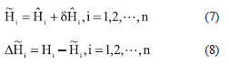
whereV_i denotes the residual of benchmark I;f(x_i,y_i) is a function which establishes the relationship between a benchmark’s and its plane coordinates. The geometric fitting methods, such as conicoid fitting method, BP neural network method, etc., can be used to determine function f(x_i,y_i).

The following data P={P₁,P₂,…,P_n}from n benchmarks are used to determine the function f(x_i,y_i).

Assume that there are n benchmarks in a test region. These n benchmarks will be divided into three categories, reference points, check points, and validation points respectively. Data from reference points, with n₁ (about 3/4 of total n benchmarks) points, will be used to determine the coefficients of the polynomial function or to train the neural network and estimate the of every reference point’s . With n2 (n2 = n – n1, about 1/4 of total n benchmarks) points, data from check points, will be used to evaluate the fitting accuracy of the determined polynomial function or the trained neural network and estimate the of every check point’s . Finally, data from validation points, with n points, will be used to estimate the of every validation point’s .

If the estimated (denoting the systematic errors of from e-GPS leveling) values of n benchmarks are available, the corrected orthometric height and corrected orthometric height difference after the first time systematic errors correction, can be calculated by equations (7) and (8) respectively.

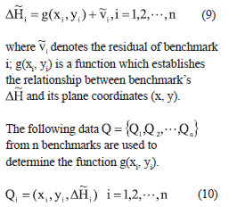
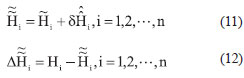
If find that there are still some systematic errors, then further assume that the following equation can express the relationship between of n benchmarks and their plane coordinates (x, y).

Again, assume that there are n benchmarks in a test region. These n benchmarks will be divided into three categories, reference points, check points, and validation points respectively. Data from reference points, with n1 (about 3/4 of total n benchmarks) points, will be used to determine the coefficients of the polynomial function or to train the neural network and estimate the of every reference point’s . With n₂ (n₂ = n – n₁, about 1/4 of total n benchmarks) points, data from check points, will be used to evaluate the fitting accuracy of the determined polynomial function or trained neural network and estimate the of every check point’s . Finally, data from validation points, with n points, will be used to estimate the of every validation point’s .

If the estimated (denoting the systematic errors of ) values of n benchmarks are available, the corrected orthometric height and corrected orthometric height difference after the second time systematic errors correction, can be calculated by equations (11) and (12) respectively.

The varied statistical values, such as mean square error, standard deviation, etc., of can be computed in the light of calculation of varied statistical values of . In addition, for simplicity, represent the standard deviations of reference points, check points, and validation points respectively.

Conicoid fitting method (CFM)

The conicoid fitting method (CFM, also known as polynomial fitting) is usually used to construct a regional geoid model (Hu et al., 2004; Hu and Sun, 2009; Lin, 2007). However, CFM will be used to estimate . The following polynomial represents the function f (xi, yi) of equation (5):

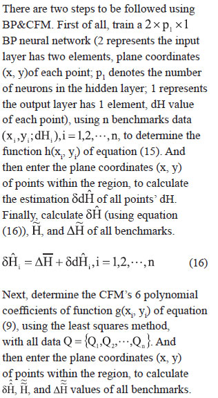
Where a₁,a₂,a₃,…denotes the undetermined coefficients of a polynomial. Three types of CFM will be tested in this paper, i.e. 4-parameter CFM (a polynomial with undetermined coefficients a₁,…,a₄), 6-parameter CFM (a polynomial with undetermined coefficients a₁,…,a₆), and 10-parameter CFM (a polynomial with undetermined coefficients a₁,…,a₁₀). When the total number of benchmarks is greater than the number of undetermined coefficients, the undetermined coefficients of a polynomial can be estimated using the least squares method. And, then enter the plane coordinates (x, y) of benchmarks within the region to equation (13), those values, such as and , after the first time systematic error correction of e-GPS leveling, can be estimated using the following CFM procedures.

BP Neural Network and BP Neural Network Method (BP&BP)

Back-propagation (BP) neural network (i.e., the multilayer feed-forward neural network), is one of the neural network algorithms. The structure of BP neural network is divided into input layer, hidden layer and an output layer.

BP neural networks are often used to construct a regional geoid model (Hu et al., 2004; Hu and Sun, 2009; Kavzoglu and Saka, 2005; Kuhar et al., 2001; Lin, 2007; Lin, 2012; Stopar et al., 2006). However, this paper will use the BP neural network and BP neural network method (BP&BP) to estimate the values of and of e-GPS leveling respectively.

First of all, a 2 X p₁ X 1 BP neural network (2 represents the input layer has two elements, plane coordinates (x, y) of each point; p1 denotes the number of neurons in the hidden layer; 1 represents the output layer has 1 element, value of each point), is trained to determine the function f (x_i, y_i) of equation (5), using n benchmarks data P={P₁,P₂,…P_n}. And then enter the plane coordinates (x, y) of points within the region, to calculate , and values of all benchmarks, after the first time systematic errors correction of e-GPS leveling.

Next, 2 X p₁ X 1 a BP neural network (2 represents the input layer has two elements, plane coordinates (x, y) of each point; p₂ denotes the number of neurons in the hidden layer; 1 represents the output layer has 1 element, value of each point), is trained to determine the function g(x_i, y_i) of equation (9), using n benchmarks data Q={Q₁,Q₂,…,Q_n}. And then enter the plane coordinates (x, y) of points within the region, to calculate , , and values of all benchmarks, after the second time systematic errors correction of e-GPS leveling.

BP Neural Network and Conicoid Fitting Method (BP&CFM)

If n benchmarks data P={P₁,P₂,…,P_n}are available, first find the mean of all points’ , using equation (2). And, then calculate the dH value of each point using the following equation.

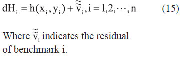
If the following equation can express the relationship between the dH values of n benchmarks and their plane coordinates (x, y).