
| Applications | |
Coverage and optimal visibilitybased navigation using visibility analysis from geospatial data
In this paper, we study the multi-sensors placement optimization problem in 3D urban environments for optimized coverage |
 |
|
 |
|
Modern cities and urban environments are becoming denser more heavily populated and are still rapidly growing, including new infrastructures, markets, banks, transportation, etc. In the last two decades, more and more cities and mega-cities have started using multi-camera networks in order to face this challenge. However, this is still not enough. Multi-sensor placement in 3D urban environments is not a simple task, also known as NP-hard one.
In this paper, we study the multi-sensors placement optimization problem in 3D urban environments for optimized coverage. The first part of our research presents a unique solution for the 3D visibility problem in built-up areas. In the second part, we present optimized coverage using multi-sensors in 3D model based on genetic algorithms using novel visibility analysis. The solutions presented in this paper can be used, among other algorithms and solutions, to enable optimal coverage and moreover optimal trajectory planning and navigation based on an optimal visibility points.
Introduction and related work
Modern cities and urban environments are becoming denser and more heavily populated and are still rapidly growing, including new infrastructures, markets, banks, transportation etc.
At the same time, security needs are becoming more and more demanding in our present era, in the face of terror attacks, crimes, and the need for improving law enforcement capabilities, as part of the increasing global social demand for efficient and immediate homeland and personal security in modern cities.
In the last two decades, more and more cities and mega-cities have started using multi-camera networks in order to face this challenge, mounting cameras for security monitoring needs [1]; however, this is still not enough [30]. Due to the complexity of working with 3D and the dynamic constraints of urban terrain, sensors were placed in busy and populated viewpoints, to observe the occurrences at these major points of interest.
These current multi-sensors placement solutions ignore some key factors, such as: visibility analysis in 3D models, which also consist of unique objects such as trees; changing the visibility analysis aspect from visible or invisible states to semi-visible cases, such as trees, and above all, optimization solutions which take these factors into account.
Multi-sensor placement in 3D urban environments is not a simple task. The optimization problem of the optimal configuration of multi sensors for maximal coverage is a well-known Non-deterministic Polynomialtime hard (NP-hard) one [5], even without considering the added complexity of urban environments.
An extensive theoretical research effort has been made over the last four decades, addressing a much simpler problem in 2D known as the art gallery problem, with unrealistic assumptions such as unlimited visibility for each agent, while the 3D problem has not received special attention [8][28][35].
The coupling between sensors’ performances and their environment’s constraints is, in general, a complex optimization problem. In this paper, we study the multi-sensors placement optimization problem in 3D urban environments for optimized coverage based on genetic algorithms using novel visibility analysis.
Our optimization solution for this problem relates to maximal coverage from a number of viewpoints, where each 3D position (x, y, z coordinates) of the viewpoint is set as part of the optimized solution. The search space contains local minima and is highly non-linear. The Genetic Algorithms are global search methods, which are well-suited for such tasks. The optimization process is based on randomly generating an initial population of possible solutions (called chromosomes) and, by improving these solutions over a series of generations, it is able to achieve an optimal solution [36].
Multi-sensor placements are scene- and application- dependent, and for this reason generic rules are not very efficient at meeting these challenges. Our approach is based on a flexible and efficient analysis that can handle this complexity.
The total number of sensors is a crucial parameter, due to the real-time outcome data that should be monitored and tracked, where too many sensors are not an efficient solution. We address the sensor numbers that should be set as a tradeoff of coverage area and logical data sources that can be monitored and tracked.
As part of our high-dimension optimization problem, we present several 3D models, such as B-ref, sweeping and wireframe models, Polyhedral Terrain Models (PTM) and Constructive Solid Geometry (CSG) for an efficient 3D visibility analysis method, integrating trees as part of our fast and efficient visibility computation, thus extending our previous work [25] to 3D visible volumes.
Accurate visibility computation in a 3D environments is a very complicated process demanding a high computational effort, which cannot be easily carried out in a very short time using traditional wellknown visibility methods [41]. The exact visibility methods are highly complex, and cannot be used for fast applications due to their long computation time. As mentioned above, previous research in visibility computation has been devoted to open environments using Digital Elevation Model (DEM) models, representing raster data in 2.5D (Polyhedral model), which do not address, or suggest solutions for, densely built-up areas.
One of the most efficient methods for DEM visibility computation is based on shadow-casting routine. The routine casts shadowed volumes in the DEM, like a light bubble [42]. Other methods related to urban design environment and open space impact treat abstract visibility analysis in urban environments using DEM, focusing on local areas and approximate openness [20]. Extensive research treated Digital Terrain Models (DTM) in open terrains, mainly Triangulated Irregular Network (TIN) and Regular Square Grid (RSG) structures. Visibility analysis on terrain was classified into point, line and region visibility, and several algorithms were introduced based on horizon computation describing visibility boundaries [11] [12].
A vast number of algorithms have been suggested for speeding up the process and reducing computation time [38]. Franklin [21] evaluates and approximates visibility for each cell in a DEM model based on greedy algorithms. An application for siting multiple observers on terrain for optimal visibility cover was introduced in [23]. Wang et al. [52] introduced a Grid-based DEM method using viewshed horizon, saving computation time based on relations between surfaces and Line Of Sight (LOS), using a similar concept of Dead-Zones visibility [4]. Later on, an extended method for viewshed computation was presented, using reference planes rather than sightlines [53].
Most of these published papers have focused on approximate visibility computation, enabling fast results using interpolations of visibility values between points, calculating point visibility with the Line of Sight (LOS) method [13]. Other fast algorithms are based on the conservative Potentially Visible Set (PVS) [16]. These methods are not always completely accurate, as they may render hidden objects’ parts as visible due to various simplifications and heuristics.
Only a few works have treated visibility analysis in urban environments. A mathematical model of an urban scene, calculating probabilistic visibility for a given object from a specific viewcell in the scene, has been presented by [37]. This is a very interesting concept, which extends the traditional deterministic visibility concept. Nevertheless, the buildings are modeled as cylinders, and the main challenges of spatial analysis and model building were not tackled. Other methods have been developed, subject to computer graphics and fields of vision, dealing with exact visibility in 3D scenes, without considering environmental constraints. Concerning this issue, Plantinga and Dyer [41] used the aspect graph – a graph with all the different views of an object. Shadow boundaries computation is a very popular method, studied by [14][47][48]. All of these works are not applicable to a large scene, due to computational complexity.
As mentioned, online visibility analysis is a very complicated task. Recently, off-line visibility analysis, based on preprocessing, was introduced. Cohen-Or et al. [4] used a ray-shooting sample to identify occluded parts. Schaufler et al. [44] use blocker extensions to handle occlusion.
Since visibility analysis in 3D urban environments is a very complicated task, it is therefore our main optimization function, known as Fitness. We introduce an extended visibility aspect for the common method of Boolean visibility values, “1” for objects seen and “0” for objects unseen from a specific viewpoint, and treat trees as semi-visibility values (such as partially seen, “0.5” value), thereby including in our analysis the real environmental phenomena which are commonly omitted.
We extend our previous work and propose fast and exact 3D visible volumes analysis in urban scenes based on an analytic solution, integrating trees into our 3D model, and it is demonstrated with a real urban scene model from Neve- Sha’anan neighborhood (within the city of Haifa).
In the following sections, we first introduce an overview of 3D models and our demands from these models. In the next section, we extended the 3D visible volumes analysis which, for the first time, takes trees into account. Later on, we present the simulation using the Neve-Sha’anan neighborhood (within the city of Haifa) 3D model. We present our genetic algorithm optimization stages and simulation based on our 3D visible volumes analysis, taking trees into account. Eventually, we extend our current visibility aspect and include conditions necessary for visibility based on the sensor’s stochastic character and present the effect of these limitations on our visibility analysis.
Analytic 3D visible volumes analysis
In this section, we present fast 3D visible volumes analysis in urban environments, based on an analytic solution which plays a major role in our proposed method of estimating the number of clusters. We briefly present our analysis presented in [27], extending our previous work [25] for surfaces’ visibility analysis, and present an efficient solution for visible volumes analysis in 3D.
We analyze each building, computing visible surfaces and defining visible pyramids using analytic computation for visibility boundaries [25]. For each object we define Visible Boundary Points (VBP) and Visible Pyramid (VP).
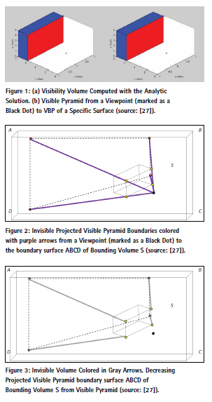
A simple case demonstrating an analytic solution from a visibility point to a building can be seen in Figure 5(a). The visibility point is marked in black, the visible parts colored in red, and the invisible parts colored in blue where VBP are marked with yellow circles.
In this section, we briefly introduce our concept for visible volumes inside bounding volume by decreasing visible pyramids and projected pyramids to the bounding volume boundary. First, we define the relevant pyramids and volumes.
The Visible Pyramid (VP): we define VPi j=1..Nsurf(x0, y0, z0 ) of object i as a 3D pyramid generated by connecting VBP of specific surface j to a viewpoint V(x0, y0, z0 ).
In the case of a box, the maximum number of Nsurf for a single object is three. VP boundary, colored with green arrows, can be seen in Figure 5(b).
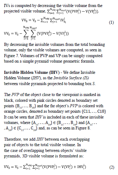
For each VP, we calculate Projected Visible Pyramid (PVP), projecting VBP to the boundaries of the bounding volume S.
Projected Visible Pyramid (PVP) – we define PVPi j..Nsurf(x0, y0, z0) of object i as 3D projected points to the bounding volume S, VBP of specific surface j through viewpoint V(x0, y0, z0). VVP boundary, colored with purple arrows, can be seen in Figure 6.
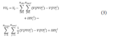
The 3D Visible Volumes inside bounding volume S, VVs, computed as the total bounding volume S, Vs minus the Invisible Volumes IVs. In a case of no overlap between buildings, IVs is computed by decreasing the visible volume from the projected visible volume, . (1) By decreasing the invisible volumes from the total bounding volume, only the visible volumes are computed, as seen in Figure 7. Volumes of PVP and VP can be simply computed based on a simple pyramid volume geometric formula.
The same analysis holds true for multiple overlapping objects, adding the IHV between each two consecutive objects.
Extended formulation for two buildings with or without overlap can be seen in [27].
Partial Visibility Concept – Trees In this research, we analyze trees as constant objects in the scene, and formulate a partial visibility concept. In our previous work, we tested trees as dynamic objects and their effect on visibility analysis [26]. Still, the analysis focused on trees’ branches over time, setting visible and invisible values for each state, taking into account probabilistic modeling in time.
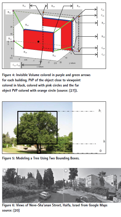
We model trees as two boxes [40], as seen in Figure 9. The lower box, bounded between [o, h1] models the tree’s trunk, leads to invisible volume and is analyzed as presented previously, for a box modeling building’s structures. On the other hand, the upper box bounded between [h1, h2] is defined as partially visible, since a tree’s leaves and the wind’s effect are hard to predict and continuously change over time. Due to these inaccuracies, we set the projected surfaces and the Projected Visible Pyramid of this box as half visible volume. According to that, a tree’s effect on our visibility analysis is divided into regular boxes included in the total number of objects, Nobj (identical to the building case), and the upper boxes modeling the tree’s leaves, denoted as Ntrees The total 3D visible volumes can be formulated as:
Simulations
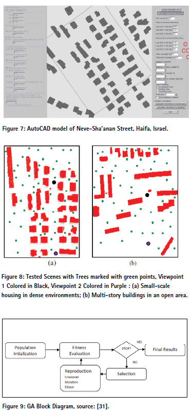
In this section, we demonstrate our 3D visible volumes analysis in urban scenes integrated with trees, presented in the previous section. We have implemented the presented algorithm and tested some urban environments on a 1.8GHz Intel Core CPU with Matlab. Neve-Sha’anan Street in the city of Haifa was chosen as a case study, presented in Figure 10.
We modeled the urban environment into structures using AutoCAD model, as seen in Figure 11, with bounding box S. By using the Matlab©MathWorks software, we automated the transformation of data from AutoCAD structure to our model’s internal data structure.
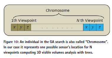
Our simulations focused on two cases: (1) small-scale housing in dense environments; (2) Multi-story buildings in an open area. These two different cases do not take the same objects into account. The first viewpoint is marked with black dot and the second one marked in purple, as seen in Figure 12. Since trees are not a part of our urban scene model, trees are simulated based on similar urban terrain in Neve-Sha’anan. We simulated fifty trees’ locations using standard Gauss normal distribution, where the trees’ parameters are defined randomly h1 ∈ (0.3,0.9), h2 ∈ (1.5,3), as seen in Figure 12.
We set two different viewpoints, and calculated the visible volumes based on our analysis presented in the previous sub-section. Visible volumes with time computation for different cases of bounding boxes’ test scenes are presented in Table II and Table III.
One can notice that the visible volumes become smaller in the dense environments described in Table II, as we enlarge the bounding box. Since we take into account more buildings and trees, less volumes are visible and the total visible volumes from the same viewpoint are smaller.
Complexity analysis
We analyze our algorithm complexity based on the pseudo code presented in the previous section, where n represents the number of buildings and trees. In the worst case, n objects hide each other. Visibility complexity consists of generating VBP and VPV for n objects, nO(1) complexity. Projection and intersection are also nO(1) complexity. The complexity of our algorithm, without considering data structure managing for urban environments, is nO(1) .
Optimized coverage using genetic algorithms
The Genetic Algorithm (GA) presented by Holland [31] is one of the most common algorithms from the evolutionary algorithms class used for complex optimization problems in different fields, such as: pharmaceutical design [33], financial forecasting [50], tracking and coverage [18][39][45], and bridge design [24]. These kinds of algorithms, inspired by natural selection and genetics, are sometimes criticized for their lack of theoretical background due to the fact that in some cases the outcome is unpredictable or difficult to verify.
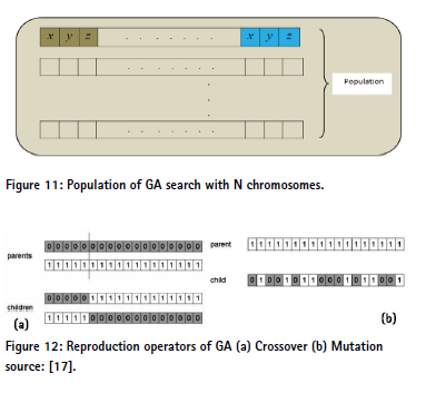
The main idea behind GA is based on repeated evaluation of individuals (which are part of a candidate solution) using an objective function over a series of generations. These series are improved over generations in order to achieve an optimal solution. In the next paragraphs, we present the genetic algorithms’ main stages, adapted to our specific problem.
The major stages in the GA process (evaluation, selection, and reproduction) are repeated either for a fixed number of generations, or until no further improvement is noted.
The common range is about 50-200 generations, where fitness function values improve monotonically [31]. A block diagram of GA is depicted in Figure 13.
Population initialization: The initialization stage creates the first generation of candidate solutions, also called chromosomes. A population of candidate solutions is generated by a random possible solution from the solution space. The number of individuals in the population is dependent on the size of the problem and also on computational capabilities and limitations. In our case it is defined as 500 chromosomes, due to the fact that 3D visible volumes must be computed for each candidate.
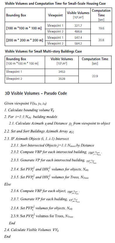
For our case, the initialized population of viewpoints configuration is set randomly, and would probably be a poor solution due to its random nature, as can be estimated. The chromosome is a 3xN-dimensional vector for N sensor’s locations, i.e. viewpoints, where position and translation is a 3-dimensional (x,y,z) vector for each viewpoint location, as seen in Figure 14. The population is depicted in Figure 15.
Evaluation: The key factor of genetic algorithm relates to individual evaluation which is based on a score for each chromosome, known as Fitness function. This stage is the most time-consuming in our optimization, since we evaluate all individuals in each generation. It should be noticed that each chromosome score leads to 3D visible volume computation N times. As a tradeoff between the covered area and computational effort, we set N to eight. In the worst case, one generation evaluation demands visibility analysis for four thousand different viewpoints. In such a case, one can easily understand the major drawback of the GA method in relation to computational effort. Nevertheless, parallel computation has made a significant breakthrough over the last two decades; GA and other optimization methods based on independent evaluation of each chromosome can nearly be computed in linear time.
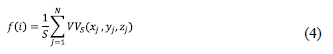
Fitness Function The fitness function evaluates each chromosome using optimization function, finding a global minimum value which allows us to compare chromosomes in relation to each other.
In our case, we evaluate each chromosome’s quality using 3D visible volumes normalized to the bounding box S around a viewpoint:
Selection: Once the population is sorted by fitness, chromosomes’ population with greater values will have a better chance of being selected for the next reproduction stage. Over the last years, many selection operators have been proposed, such as the Stochastic Universal Sampling and Tournament Selection. We used the most common Tournament, where k individuals are chosen randomly, and the best performance from this group is selected. The selection operator is repeated until a sufficient number of parents are chosen to form a child generation.
Reproduction: In this stage, the parent individuals chosen in the previous step are combined to create the next generation. Many types of reproduction have been presented over the years, such as crossover, mutation and elitism.
Crossover takes parts from two parents and splices them to form two offspring, as seen in Figure 16(a). Mutation modifies the parameters of a randomly selected chromosome from within a single parent, as seen in Figure 16(b). Elitism takes the fittest parents from the previous generation and replicates them into the new generation. Finally, individuals not selected as parents are replaced with new, random offspring. Further analysis and operators can be found in [29][36]. The major steps of these operators can be seen in Figure 16.
Simulations
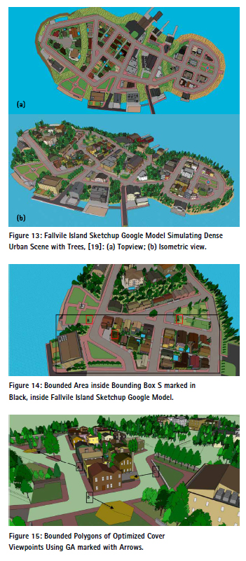
In this section, we report on simulation runs with our 3D visible volumes analysis in urban scenes integrated with trees, using genetic algorithms. The genetic algorithms were tested on a 1.8GHz Intel Core CPU with Matlab. We used Fallvile Island Sketchup Google Model [19] for simulating a dense urban scene with trees, as seen in Figure 17.
The stages of Crossover and Elitism operators are described as follows, with a probability of Pc=0.9 (otherwise parents are copied without change):
1. Choose a random point on the two parents
2. Split parents at this crossover point
3. Create next generation chromosomes by exchanging tails
Where the Mutation operator modifies each gene independently with a probability of Pm=0.1
In order to process the huge amount of data, we bounded a specific region which includes trees and buildings, as seen in Figure 18. We imported the chosen region to Matlab and modeled the objects by boxes, neglecting roofs’ profiles. Time computation for one generation was one hour long on average. As we could expect, the evaluation stage took up 94% of the total simulation time. We set the bounding box S as [500 m* 200 m* 50 m]. Population initialization included 500 chromosomes, each of which is a 24-dimensional vector consisting of position and translation, where all of them were generated randomly.
Based on the Fitness function described previously and the different GA stages and 3D visible volumes analysis, the location of eight viewpoints for sensor placement was optimized. Viewpoints must be bounded in S and should not penetrate buildings and trees. Stop criteria was set to 50 generations and Fitness function gradient.
Optimal coverage of viewpoints and visible volumes during ten runnings’ simulations is seen in Figure 19, bounded in polygons marked with arrows. During these ten runnings simulations, we initialized the population randomly at different areas inside bounding box S.
These interesting results show that trees’ effect inside a dense urban environment was minor, and trees around the buildings in open spaces set the viewpoint’s location. As seen in Figure 19, polygon A and polygon B are both outside the areas blocked by buildings. But they are still located near trees, which affect the visible volumes, and we can predict that the same affect will occur in our real world. On the other hand, polygon C, which is closer to the area blocked by buildings, takes into account the trees in this region, but the major factor are still the buildings.
Conclusions
In this paper, we presented an optimized solution for the problem of computing maximal coverage from a number of viewpoints, using a genetic algorithms method. In addition, we propose the conditions necessary for visibility based on sensors’ model analysis, taking into account stochastic character. As far as we know, for the first time we integrated trees as partially visible objects participating in a 3D visible volumes analytic analysis and conditions necessary for visibility with sensors’ noises effects. As part of our research we tested several 3D models of 3D urban environments from the visibility viewpoint, choosing the best model from the computational effort and the analytic formulation aspects.
We tested our 3D visible volumes method on real a 3D model from an urban street in the city of Haifa, with time computation and visible volumes parameters.
In the second part of the paper, we introduced a genetic algorithm formulation to calculate an optimized solution for the visibility problem. We used several reproduction operators, which made our optimization robust. We tested our algorithm on the Fallvile Island Sketchup Google Model combined with trees, and analyzed the viewpoint’s polygons results, and also compared using versus not using the conditions necessary for visibility. Based on our results, an optimal trajectory can be planned by using an optimal visibility points as basic global search results, adding local permutations over it.
Our future work is related to validation between our simulated solution and projected volumes from sensors mounted in these viewpoints for optimal coverage.
References
[1] O. Gal and Y. Doytsher, “Sensors Placement in Urban Environments Using Genetic Algorithms,” The Senventh International Conference on Advanced Geographic Information Systems, Applications, and Services, pp. 82-87, 2015.
[2] N. Abu-Akel, “Automatic Building Extraction Using LiDAR Data,” PhD Dissertation, Technion, Israel, 2010.
[3] D. Cohen-Or, G. Fibich, D. Halperin and E. Zadicario, “Conservative Visibility and Strong Occlusion for Viewspace Partitioning of Densely Occluded Scenes,” In EUROGRAPHICS’98.
[4] D. Cohen-Or and A. Shaked, “Visibility and Dead- Zones in Digital Terrain Maps,” Eurographics, vol. 14, no. 3, pp.171-180, 1995.
[5] R. Cole and M. Sharir, “Visibility Problems for Polyhedral Terrain,” Journal of Symbolic Computation, vol. 7, pp.11-30, 1989.
[6] K. Chakrabarty, S. Iyengar, H. Qi and E. Cho, “Grid Coverage for Surveillance and Target Location in Distributed Sensor Networks,” IEEE Trans. Comput, vol. 51, no. 12, 2002.
[7] Y. Chrysanthou, “Shadow Computation for 3D Interactive and Animation,” Ph.D. Dissertation, Department of Computer Science, College University of London, UK, 1996.
[8] R. Church and C. ReVelle, “The Maximal Covering Location Problem,” Papers of the Regional Science Association, vol. 32, pp.101-118, 1974.
[9] T. Clouqueur, V. Phipatanasuphorn, P. Ramanathan and K.K. Saluja, “Sensor deployment strategy for target detection,” In WSNA, 2002.
[10] T. Clouqueur, K.K. Saluja and P. Ramanathan, “Fault tolerance in collaborative sensor networks for target detection,” IEEE Trans. Comput, vol. 53, no. 3, 2004.
[11] L. De Floriani and P. Magillo, “Visibility Algorithms on Triangulated Terrain Models,” International Journal of Geographic Information Systems, vol. 8, no. 1, pp.13-41, 1994.
[12] L. De Floriani and P. Magillo, “Intervisibility on Terrains,” In P.A. Longley, M.F. Goodchild, D.J. Maguire & D.W. Rhind (Eds.), Geographic Information Systems: Principles, Techniques, Management and Applications, pp. 543-556. John Wiley & Sons, 1999.
[13] Y. Doytsher and B. Shmutter, “Digital Elevation Model of Dead Ground,” Symposium on Mapping and Geographic Information Systems (ISPRS Commission IV), Athens, Georgia, USA, 1994.
[14] G. Drettakis and E. Fiume, “A Fast Shadow Algorithm for Area Light Sources Using Backprojection,” In Computer Graphics (Proceedings of SIGGRAPH ’94), pp. 223–230, 1994.
[15] M.F. Duarte and Y.H. Hu, “Vehicle classification in distributed sensor networks,” Journal of Parallel and Distributed Computing, vol. 64, no. 7, 2004.
[16] F. Durand, “3D Visibility: Analytical Study and Applications,” PhD thesis, Universite Joseph Fourier, Grenoble, France, 1994.
[17] A.E. Eiben and J.E. Smith, “Introduction to Evolutionary Computing Genetic Algorithms,” Lecture Notes, 1999.
[18] U.M. Erdem and S. Sclaroff, “Automated camera layout to satisfy task- specific and floor plan-specific coverage requirements,” Computer Vision and Image Understanding, vol. 103, no. 3, pp. 156–169, 2006.
[19] Fallvile, (2010) http://sketchup. google.com/3dwarehouse/ details?mid =2265cc05839f0e5925ddf6e8265 c857c&prevstart=0
[20] D. Fisher-Gewirtzman, A. Shashkov and Y. Doytsher, “Voxel Based Volumetric Visibility Analysis of Urban Environments,” Survey Review, DOI: 10.1179/1752270613Y. 0000000059, 2013.
[21] W.R. Franklin, “Siting Observers on Terrain,” in D. Richardson and P. van Oosterom, eds, Advances in Spatial Data Handling: 10th International Symposium on Spatial Data Handling. Springer-Verlag, pp. 109-120, 2002.
[22] W.R. Franklin and C. Ray, “Higher isn’t Necessarily Better: Visibility Algorithms and Experiments,” In T. C. Waugh & R. G. Healey (Eds.), Advances in GIS Research: Sixth International Symposium on Spatial Data Handling, pp. 751-770. Taylor & Francis, Edinburgh, 1994.
[23] W.R. Franklin and C. Vogt, “Multiple Observer Siting on Terrain with Intervisibility or Lores Data,” in XXth Congress, International Society for Photogrammetry and Remote Sensing. Istanbul, 2004.
[24] H. Furuta, K. Maeda and E. Watanabe, “Application of Genetic Algorithm to Aesthetic Design of Bridge Structures,” Computer-Aided Civil and Infrastructure Engineering, vol. 10, no. 6, pp.415–421, 1995.
[25] O. Gal and Y. Doytsher, “Analyzing 3D Complex Urban Environments Using a Unified Visibility Algorithm,” International Journal On Advances in Software, ISSN 1942-2628, vol. 5 no.3&4, pp:401-413, 2012.
[26] O. Gal and Y. Doytsher, “Dynamic Objects Effect on Visibility Analysis in 3D Urban Environments,” Lecture Notes in Computer Science (LNCS), vol. 7820, pp.147- 163, DOI 10.1007/978-3-642- 37087-8_11, Springer, 2013.
[27] O. Gal and Y. Doytsher, “Spatial Visibility Clustering Analysis In Urban Environments Based on Pedestrians’ Mobility Datasets,” The Sixth International Conference on Advanced Geographic Information Systems, Applications, and Services, pp. 38-44, 2014.
[28] H. Gonz ́alez-Ban ̃os and J.C. Latombe, “A randomized art-gallery algorithm for sensor placement,” in ACM Symposium on Computational Geometry, pp. 232–240, 2001.
[29] D.E. Goldberg and J.H. Holland, “Genetic Algorithms and Machine Learning,” Machine Learning, vol. 3, pp.95-99, 1998.
[30] Holden (2013), http:// slog.thestranger.com/slog/ archives/2013/04/21/after-theboston- bombings-do-american-citiesneed- more-surveillance-cameras
[31] J. Holland, “Adaptation in Natural and Artificial Systems,” University of Michigan Press, 1975.
[32] D. Li and Y.H. Hu, “Energy based collaborative source localization using acoustic micro-sensor array,” EUROSIP J. Applied Signal Processing, vol. 4, 2003.
[33] D. Maddalena and G. Snowdon, “Applications of Genetic Algorithms to Drug Design,” In Expert Opinion on Therapeutic Patents, pp. 247-254, 1997.
[34] M. Mäntylä M, “An Introduction to Solid Modeling,” Computer Science Press Rockville, Maryland, 1988.
[35] M. Marengoni, B.A. Draper, A. Hanson and R. Sitaraman, “A System to Place Observers on a Polyhedral Terrain in Polynomial Time,” Image and Vision Computing, vol. 18, pp.773-780, 2000.
[36] M. Mitchell, “An Introduction to Genetic Algorithms (Complex Adaptive Systems),” MIT Press, 1998.
[37] B. Nadler, G. Fibich, S. Lev-Yehudi D. and Cohen-Or, “A Qualitative and Quantitative Visibility Analysis in Urban Scenes,” Computers & Graphics, vol. 5, pp.655-666, 1999.
[38] G. Nagy, “Terrain Visibility, Technical report,” Computational Geometry Lab, ECSE Dept., Rensselaer Polytechnic Institute, 1994.
[39] K.J. Obermeyer, “Path Planning for a UAV Performing Reconnaissance of Static Ground Targets in Terrain,” in Proceedings of the AIAA Guidance, Navigation, and Control Conference, PP.1-11, 2009.
[40] K. Omasa, F. Hosoi, T.M. Uenishi, Y. Shimizu and Y. Akiyama, “Three-Dimensional Modeling of an Urban Park and Trees by Combined Airborne and Portable On-Ground Scanning LIDAR Remote Sensing,” Environ Model Assess vol. 13, pp.473–481, DOI 10.1007/s10666-007-9115-5, 2008.
[41] H. Plantinga and R. Dyer, “Visibility, Occlusion, and Aspect Graph,” The International Journal of Computer Vision, vol. 5, pp.137-160, 1990.
[42] C. Ratti, “The Lineage of Line: Space Syntax Parameters from the Analysis of Urban DEMs,” Environment and Planning B: Planning and Design, vol. 32, pp.547-566, 2005.
[43] H. Samet, “Hierarchical Spatial Data Structures,” Symposium on Large Spatial Databases (SSD), pp. 193-212, 1989.
[44] G. Schaufler, J. Dorsey, X. Decoret and F.X. Sillion, “Conservative Volumetric Visibility with Occluder Fusion,” In Computer Graphics, Proceedings of SIGGRAPH, pp. 229-238, 2000.
[45] V. Shaferman and T. Shima, “Coevolution genetic algorithm for UAV distributed tracking in urban environments,” in ASME Conference on Engineering Systems Design and Analysis, 2008.
[46] A. Streilein, “Digitale Photogrammetrie und CAAD,” Ph.D Thesis, Swiss Federal Institute of Technology (ETH) Zürich, Diss. ETH Nr. 12897, Published in Mitteilungen Nr. 68 of the Institute of Geodesy and Photogrammetry, 1999.
[47] J. Stewart and S. Ghali, “Fast Computation of Shadow Boundaries Using Spatial Coherence and Backprojections,” In Computer Graphics, Proceedings of SIGGRAPH, pp. 231-238, 1994.
[48] S.J. Teller, “Computing the Antipenumbra of an Area Light Source,” Computer Graphics, vol. 26, no.2, pp.139-148, 1992.
[49] D. Tian and N.D. Georganas, “A coverage-preserved node scheduling scheme for large wireless sensor networks,” In WSNA, 2002.
[50] E.P.K. Tsang and J. Li, “Combining Ordinal Financial Predictions with Genetic Programming,” In Proceedings of the Second International Conference on Intelligent Data Engineering and Automated Learning, pp. 532–537, 2000.
[51] P. Varshney, “Distributed Detection and Data Fusion,” Spinger-Verlag, 1996.
[52] J. Wang, G.J. Robinson and K. White, “A Fast Solution to Local Viewshed Computation Using Grid-based Digital Elevation Models,” Photogrammetric Engineering & Remote Sensing, vol. 62, pp.1157-1164, 1996.
[53] J. Wang, G.J. Robinson and K. White K, “Generating Viewsheds without Using Sightlines,” Photogrammetric Engineering & Remote Sensing, vol. 66, pp. 87-90, 2000.
The paper was prepared for presentation at the “2020 WORLD BANK CONFERENCE ON LAND AND POVERTY” The World Bank – Washington DC, March 16-20, 2020.


 (No Ratings Yet)


Leave your response!