Mine planning and design

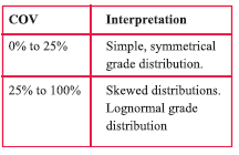
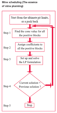
Introduction

The mine site is located in district Raipur in the state of chattisgarh. Geologically, this mine predominantly contains limestone of marginal to sub-marginal grade. The mine has been explored at a grid interval of 100/ 200 meters at a sampling interval of 0.5-meter along depth. Moreover as the water table is very shallow in the area, core cum sludge samples were taken to improve the reliability of the samples. Structurally, the area contains massive limestone of grey/ purple/ chocolate in color very well differentiated from a separate 2 – 3 meters of boundary limestone formation mixed with soil and buff shale. The massive limestone band contains cryptocrystalline shale partings, which cannot be segregated to a much greater extent by scrubbing, screening, magnetic separation, or any other benefi ciation techniques generally used. This made the mine more vulnerable for proper and judicious mine planning so as sustain the mine in terms of quantity and quality deliverables over a longer period. Hence a need was felt to redesign the geological model of our mine with proper estimation using surpac and total station to best fi t our mining requirements.

Computerized mine planning

It was felt that the geological and the block model of the mine has to be relooked upon in-house using surpac. Before moving a further one-step ahead let us think upon the probable sources that can lead us to such errors.

a) Lack of a well-defi ned geological model.

b) Lack of proper inputs/ basis for calculating the block estimates.

As the data has been entered by two different agencies and it was observed that there was not much of differences between the two, it was assumed that error in this stage is zero or negligible.

Re-defi ning the geological model

All the geological models designed earlier were more or less literally based on the extent of lithology. But during the course of winning limestone it is a normal practice that the loader/ excavator operator segregates the inter-burden/ waste material from the blasted muck and feeds the remaining material to a crusher. Hence, it is very relevant that in order to resemble our geologic model to the field, it has to be categorized assay wise in term of a specific radical. This paved the way that an assay bearing area containing on an average 41% lime and above can be a best fit domain to meet our requirements and same was done accordingly.

Basic statistics

After re-defiing the geological model, basic statistics of important adicals were computed to calculate the following –

1. Average grade (mean).

2. Standard deviation (std. dev.).

3. Coefficient of variation (COV).

On detailed analysis of the coeffi cient of variation of the respective adicals, following interpretation were derived on the basis of below mentioned generally followed norms.

It was thereupon interpreted that excepting CaO, most of the other radicals followed a lognormal distribution.

Variogram modeling

The variogram is the fundamental tool used to measure spatial continuity of grade data and is a plot between average variability between samples vs. the distance between samples.

Computing an experimental variogram

Computing an experimental variogram from a set of randomly spaced data involves fi nding pairs of data that are oriented in the required direction, determining the distance between the samples, then summing the squared differences of the grades. Since the data are usually sparse, it is necessary to use a tolerance when locating samples in the desired direction and to use a distance increment to classify samples by distance. The distance tolerance is a fixed distance increment (cell size), selected so a reasonable number of samples fall in each cell. The steps/ procedures observed by us to compute the experimental variogram is detailed below –

1. Variograms were computed within continuous zones of mineralization without crossing different geologic domains.

2. The distance increment was approximately equal to the average spacing between samples in the direction of the variogram.

3. At least 30 pairs of samples were used to compute a valid variogram.

Resource estimation

The generally used methods for resource estimation or modeling are –

1. Traditional/ geometric methods that are done manually on plans or sections and

2. Interpolation methods such as inverse-distanceweighting and kriging that require the use of a computer.

Kriging

Kriging is the geostatistical estimation method developed to provide the “best linear, unbiased estimate” for grade based on a least squares minimization of the error of estimation, or kriging error. Important factors in the krigging estimate are

1. The average of the estimates should not be systematically higher or lower that the truevalue; this is established mathematically by setting sum of weights equal to zero.

2. The error of estimation, which is expressed as krigged variance is minimized using the lagrange principle to create a moidified equation that satisfies a non-bias constant, called as lagrange multiplier.

3. The equation is then differentiated with respect to each of the weights & lagrange multiplier resulting in a set of simultaneous equations.

4. The simultaneous equation is then solved by gaussian elimination method to determine the weights and lagrange multiplier.

5. The krigging error of estimation is there upon computed.

6. The individual variance of samples in the deposit and the block variances can be thereupon computed from the experimental variogram.

Following precautions were taken to facilitate the krigging process:

Block size

1. With the existing spacing of minimum 100 meters between holes a block size of ¼ th of the drill hole spacing was taken.

Sample selection

1. Samples were selected from geologic domain similar to the block

2. To avoid overestimation as well as under estimation a min-max of 10 – 20 samples were only taken.

Step – 1

Find the cone value for each ore block (positive block) within a given pushback, or within the ultimate pit limits. For this, the apex of a cone is set over each ore block, and the economic values of all the ore and waste blocks that are within the cone and have to be mined before mining the block at the apex are summed. This total economic value of a given block , I, is said to be the cone value of the block i, Cvi.

Step – 2

Assign the co-efficients to the ore blocks according to their cone value, which may also be considered as a ranking of the core blocks by bench. On the uppermost bench where one or more ore blocks exists,

1 is assigned to the ore block with the highest cone value ,

2 is assigned to the ore block with the second highest cone value, and so on. If there are three ore blocks on that bench,

3 is assigned to the ore block with the smallest cone value. Then the ranking process moves one bench down. If there are some ore blocks on that bench,

4 is assigned to the ore block with the highest cone value. The process is performed for all the ore blocks within a given pushback. If two ore blocks on the same bench have the same cone value, the co-effi cients are assigned randomly, and two ore blocks should not be assigned the same co-effi cient.

Step – 3

Set up an LP formulation to generate the FTs, as detailed in the next session. When the problem formulation is complete, any solver suitable for large models may be used to solve it.

Step – 4

If the number of trees obtained is the same as the number of the trees obtained from the previous solution, the solution is considered to be optimal, and the algorithm can go to the next step. If the number of trees is higher than the previous solution, keep the currently found connections between blocks and repeat all the steps as illustrated in the next section. Initially, just for being theoretical correct, assume that whole pushback is one tree.

Step – 5

Stop the algorithm.

Observations

It was observed that the estimates were now more or less tallying with the actual achieved grades. In order to further streamline the same it was further decided to experiment use of blast hole drill samples for more localized estimates and then establishing the deviations.

I express my sincere thanks to the management of Grasim Cement for allowing me to publish the paper. The views expressed in this paper are solely of the author and not necessarily of the management.

References

(1) Fundamental tree algorithm in optimising production scheduling for open pit mine design by S. Ramazan, K. Dagdelen and T. B. Johnson