
| GNSS | |
GNSS Constellation Specific Monthly Analysis Summary: September 2026
The analysis performed in this report is solely the author’s work and his opinion. |
 |
|
Introduction
This article continues the monthly performance analysis of the GNSS/SBAS constellation. Readers are encouraged to refer to previous issues for foundational discussions and earlier results. The focus for this month’s issue is the atomic time generation based on filtering and prediction. A sample data from BIPM learning platform is used to demonstrate how clock ensemble produces atomic time that can be the national laboratory time or the GNSS system time. It is solely for educational purposes.
1. Atomic Timescale Generation: Prediction Based Algorithm
In our previous analysis, we explored how a localized atomic timescale (Temps Atomique – TA) or UTC(k) is realized via a classic weighted average of an ensemble of atomic clocks. While weighted averaging can optimize the performance balance between high-short-term-stability Hydrogen Masers and robust-long-term-stability Cesium standards, it is acutely vulnerable to phase steps, clock drift, and data dropouts. If a clock suffers a sudden discontinuity, the unmitigated step maps directly into the averaged timescale, corrupting real-time synchronization networks.
To mitigate these instabilities, modern timing laboratories and GNSS control segments employ prediction-based timescale algorithms. By shifting from instantaneous averaging to forward-predictive models, the ensemble establishes an anomaly-resistant reference. This article details the structural working principles of the prediction algorithm provided by the BIPM E-Learning platform (Timescale Algorithms and their Applications), explains the critical selection criteria for predictive estimation spans, and interprets the performance results derived from the simulation script.
2. Working Principle
Phase 1: Pre-calculation of Inter-Clock Differences.
Rather than analyzing clocks in isolation, the concept calculates the differential phase offsets between a designated reference clock (clk_0, where flg == 1) and all other clocks in the ensemble: Δx_i(t) = x_0(t) – x_i(t). This eliminates common-mode laboratory noise and establishes a baseline matrix of inter-clock drift.
Phase 2: Frequency Rate Estimation and Forward Prediction.
For every designated Modified Julian Date (MJD), it predicts the tomorrow-phase (x_hat) of each clock using historical memory. The frequency rate (slope) is estimated by tracking the clock’s behavior over a predefined historical window, termed the rate estimation span (T_span): Slope = [x(t_-1) – x(t_-(T_span+1))] / [t_-1 t_-(T_span+1)]. The forward-predicted phase for the next epoch is then calculated linearly: x_hat(t) = x(t_-1) + Slope * (t -t_-1).
Phase 3: Robust Error Gating and Weighted Realization.
Before executing the ensemble average, it performs an outlier rejection check. It evaluates the deviation between a clock’s actual measured phase (df_x) and its forward-predicted phase (x_hat) against a strict threshold limit (x_limit): |x_hat(t) – df_x(t)| < x_limit.
- If the clock passes, its preset weight is included in the scale normalization.
- If a clock undergoes a phase jump or data missing anomaly, the algorithm automatically sets its effective weight to 0.0 for that day, isolating the fault.
- The clean, weighted differences are then aggregated to yield the final continuous UTCk-TA scale.
3. Selecting the Rate (Frequency) Estimation
The choice of the rate estimation span (T_span) directly governs the operational focus and noise-filtering capability of the prediction algorithm. Two primary spans are evaluated depending on the metrological or synchronization intent:
• The 10-Day Prediction Span (T_span = 10): A short history focus is optimized for systems dominated by high-quality Hydrogen Masers. Masers provide superlative short-term stability but exhibit long-term frequency drift. A tight 10-day estimation window allows the algorithm to rapidly adapt to changing drift profiles, keeping the forward prediction accurate over short horizons. However, this short span is more susceptible to high-frequency measurement noise.
• The 90-Day Prediction Span (T_span = 90): A long history focus is designed to capture the structural aging parameters of Cesium frequency standards. Cesium clocks are noisier day-to-day but highly stable over months. Extending the rate span to 90 days effectively smooths out random white phase noise, isolating the true linear deterministic drift of the ensemble. This long horizon acts as a stabilizing flywheel, though it takes longer to recover if baseline clock parameters shift permanently.
4. Results and Interpretation
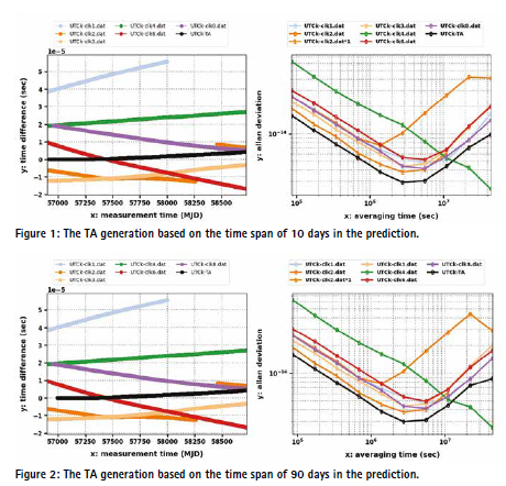
The output of the prediction script is visualized through the time-difference phase evolution plot (left) and the corresponding overlapping Allan Deviation (ADEV) stability profile (right).
Phase Evolution Analysis (Left Plot): The left plot illustrates the phase progression of the individual clocks alongside the generated composite timescale, UTCk-TA (plotted as the thick black line).
• Drift Compensation: Clocks such as clk1 (blue trace running high) and clk6 (red trace diving down) exhibit strong, uncompensated linear frequency offsets. Despite these heavy trajectories, the UTCk-TA scale remains robustly bounded near zero, demonstrating that the algorithm successfully forecasts and subtracts these systemic drifts.
• Anomaly Isolation (clk2): A severe discontinuity is visible on the orange trace of clk2 around MJD 58400, followed by a data gap and a subsequent segment labeled UTCk-clk2.dat*1. In a standard averaging scale, this sharp phase drop would drag the entire ensemble down. Because the prediction algorithm recognized that the measured phase breached the x_limit relative to its 10-day history, clk2 was dynamically de-weighted. As a result, the black UTCk-TA line continues smoothly without any visible phase step or jump.
Stability Analysis via Allan Deviation (Right Plot): The right plot characterizes the fractional frequency stability across various averaging times (τ).
• Maser vs. Cesium Structural Signatures: The active clocks exhibit distinct noise slopes. Clocks like clk3 show excellent short-term stability that degrades at longer integration times (τ > 10^6 seconds) due to unsteered drift. Conversely, the classic Cesium-type signatures (clk4) display a continuous downward slope, demonstrating superior long-term performance at large averaging times.
• Ensemble Optimization: The core success of the script is proven by the UTCk-TA stability trace (black line with circles). At short averaging times (τ = 10^5 s), it traces the low-noise floor of the best masers. As integration time increases toward τ = 10^6 s, it drops significantly below the individual Allan deviation curves of the constituent clocks. The predictive steering ensures the timescale inherits the optimal white frequency noise reduction of the combined ensemble while filtering out individual hardware artifacts.
5. Conclusion
The transition from a pure instantaneous weighted average to a prediction-based timescale algorithm represents a fundamental paradigm shift in high-precision timekeeping and metrology. By coupling historical frequency rate estimation windows—such as 10-day or 100-day observation horizons—with strict statistical error gating, the ensemble framework successfully insulates the generated timescale from real-world hardware vulnerabilities. Rather than permitting a sudden phase step or clock dropout (such as the discontinuity witnessed in clk2) to contaminate the reference, the algorithm dynamically de-weights failing components based on deviation boundaries relative to forward predictions. This structural resilience achieves a highly stable composite baseline (UTCk-TA) that inherits the optimal short-term performance of Hydrogen Masers and the robust long-term drift profile of Cesium standards.
Crucially, this mathematical «paper clock» does not merely exist as digital database coordinates. In operational timing laboratories and GNSS control stations, the calculated numerical corrections are pushed in real time to a physical hardware control loop. By utilizing an online State-Space Kalman Filter to isolate multi-component noise, a digital controller translates the paper clock’s trajectory into precise tuning parameters. These parameters drive hardware microsteppers that continuously adjust the phase of a physical Master Clock, bridging the gap between abstract algorithmic modeling and the generation of a continuous, highly synchronized 1 PPS physical signal. For modern satellite networks, this continuous, steered synchronization underpins global positioning systems, ensuring that local clock replacements or orbital anomalies remain completely invisible to the end-user.
Data sources and Tools:
https://webtai.bipm.org/database/canvas_gnss.html
Allantools, Python
elearning, BIPM, Timescale Algorithms and their Applications
Software: https://github.com/TheBIPM/Time_scale_course_material







Leave your response!