| Mapping | |
The 3rd dimension
|
||||
|
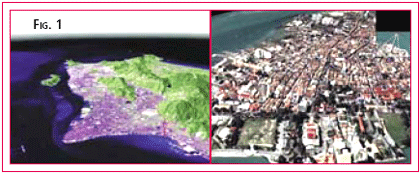
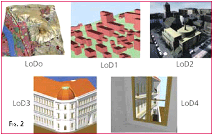
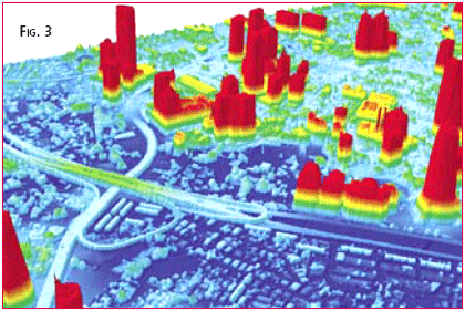
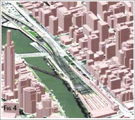
Spatial data is the fuel for 3D Applications, but all too often the fuel supplied is inappropriate. The software applied and expertise required when modelling a flood event or predicting a cityscape’s lineof-site is exactly the same using highly precise data as it is for generalised data. The difference is in how well that analysis relates to the real world … i.e. whether the analysis is correct or not. Conversely, supplying highly accurate or dense data to a generalised analysis can cost both time and money which is not reflected in the final product. Hence the word of this paper is: appropriate. Apply the most appropriate data to your application. There is nothing wrong with “approximate” or “inexpensive” 3D data, as long as it is appropriate for the level of analysis being performed. After reviewing four major components of a dataset’s composition, a number of recent case studies are offered. Finding Appropriate DataThe authors contend that there are four characteristics of a dataset which define its suitability for a 3D application, viz. resolution, accuracy, currency and format. Each is discussed briefly in turn. ResolutionResolution refers to the density of information available. In ‘the old days”, it was best summed up as the “scale” of the material under consideration. Everyone accepted that you could not do detailed design from a 1:20,000 mapsheet, or hope to see manhole covers on 1:80,000 photography. These concepts still apply to the Digital era, even though the concept of scale has been reduced to the field one enters in the PRINT window. This concept is best illustrated on two visualisations recently completed to support the Penang Outer Ring Road project. The first example is a regional dataset using Landsat imagery and SRTM surface heights (Fig 1 left). Resolution of Landsat is 30m and SRTM 90m spacing … both quite coarse but sufficient for regional analysis and often available from existing archives. The higher resolution version (Fig 1 right) involves Digital Globe imagery (at 0.6m resolution) and LiDAR surface heights (at 1m resolution). This higher resolution allows visualisation and analysis at the building-by-building level. In these cases, the resolution of the two datasets was paired well. Draping a high resolution image over low resolution surface model would have resulted in an incorrect heighting of the pixels; draping a low resolution image over a high resolution surface model would have meant the longer processing times and LiDAR capture costs were not fully returned to the project. Resolution in the context of a built environment was well described and quantified by Kolbe and Bacharach (2006), shown in Fig 2. The five “Levels of Detail (LoD)” show how the resolution (or definition) in a building can vary from a generalized outline, to intricate components. AccuracyErrors in spatial data are to be understood and enjoyed. Here is a news flash to many readers: every spatial dataset has errors. A detailed engineering survey will have errors at the millimetre level; a spatial dataset over the country will have errors at the metre level. The science of surveying is to understand the project’s “error budget” and arrive at a dataset with accuracy appropriate for its intended use. (The corollary to this is to insist that every dataset you receive comes with a metadata statement recording the accuracy and other characteristics of the dataset. A regional dataset accurate to a few metres is fine for conceptual planning, but you don’t want this data ending up in the hands of the engineers who set about detailed design work). Another news flash to readers might be that it is impossible to say how accurate every point or pixel is in your dataset. In statistical terms, data measuring is subject to random errors. Therefore it is impossible to say that “every point is accurate to 0.2m”. Because measuring and surveying are subject to the laws of statistics, surveyors rely on statistical measures to describe how accurate the dataset is. The common term to describe a dataset is “root mean square” error or “rms”. Other terminology for the same measure is “rmse”, “onesigma”, “1s” or “standard error”. What this concept means is that if you see a statement saying that “The vertical accuracy of this dataset is 0.2m rms”, it means that if you compared every point or pixel in the dataset with the truth (if somehow that were possible), then 68% of points would be within ±0.2m of the truth. The reason to use appropriately accurate data is clear to all. What is not so clear is that the work of the engineer or the effort of the visualisation specialist is generally the same regardless of the level of accuracy of the data. It is only when the flood study or the line-of-sight calculation is put back into the field and compared with reality is the quality of the underlying spatial data truly revealed. In projects involving 3D visualisation, especially in built environments, the issue of accuracy often extends to whether the buildings are defined in the application by measurement or estimation. Estimation techniques include positioning the buildings from tourist maps, estimating from imagery, or simply from memory. Building heights can be estimated by memory, reference to known heights or by counting floors. All of these estimation techniques are valid, as long as the resulting accuracy level is commensurate with the project aims. In many cases, it separates whether the project is one of “actual” or “schematics”. CurrencyCurrency refers simply to the date at which the information was captured. Decisions relating to currency typically involve assessing the relevance of off-the-shelf data, compared with the costs involved in acquiring current data specifically for your project. Acquiring current data also brings the advantage of setting resolution, accuracy and format for your project, instead of inheriting them from data acquired for other purposes. Currency can also be complicated when datasets are compiled from multiple-epochs. FormatFormat refers to the characteristics of the dataset (eg. grid, point or vector) and is often linked to the means of data capture and/or the extent of the dataset. The differences between formats are best illustrated in a built environment. The most cost-effective means of defining a cityscape is by employing the mass-points measuring technique of LiDAR (or Airborne Laser Scanning). This technique measures a dense array of accurate 3D spot elevations across the cityscape. Typical point spacing is sub-metre, with some cityscape projects in Europe now employing point spacings of a few decimetres. A LiDAR point measurement of a city defines the building height and position accurately, but the level of detail (or cartographic appeal) is relatively low. The image shown in Fig 3 is of a recent LiDAR survey of Kuala Lumpur; it illustrates the high spatial integrity but low cartographic appeal of the mass-point format. 3D-Vectors provide the most rigorous means of defining a cityscape. Typically they are obtained by stereodigitising building outlines from overlapping aerial photography. As it is a manual task, the stereooperator can pick and choose which polygons or building features needed to adequately define the building shape and appearance. The benefit of Vectors is that they provide a crisp definition of the building. Software can then extrude the 3D vectors down to the ground level to give the appearance of more lifelike structures (shown in Fig 4, from Melbourne, Australia). Because it is a manual process, costs are directly proportional to the number of buildings, and number or elements within each building, are required. SummarisingWhen deciding whether a dataset is appropriate, one needs to consider its resolution, accuracy, currency and format. Assessing the data requirements for each project will raise a series of choices. For example, a vector definition of a cityscape will look more lifelike, but it may be far less accurate than a points definition. If you have to make a choice, would you want the buildings to be lifelike or in their correct position ? You can have both, but at a significantly higher cost. Does your project warrant that investment ? On another project, you might be presented with low resolution current imagery, or high resolution archive imagery. You will have to decide whether the recent changes to the project site will detract from the information extracted from the dataset. Whatever the decision on how you assess these variables and specify your dataset, it is vital to document these characteristics so future users know the true attributes of the dataset. |
||||
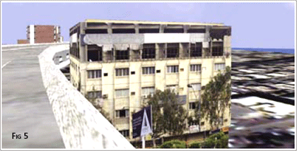
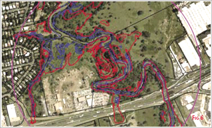
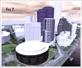
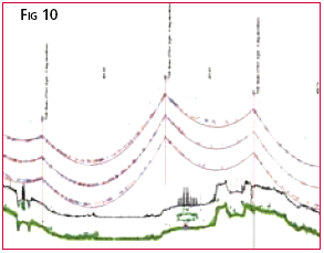
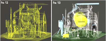
Applying Appropriate DataThe following section provides a few recent case studies with which the authors have been involved when asked to provide suitable height data to a 3D GIS. Case Study 1 – 3D Visualisation of Elevated RoadwayThis project involved the visualisation of a proposed elevated roadway in Karachi. The roadway is to be built along an existing corridor between multi-story buildings. The task was to illustrate the visual impact of the roadway on the cityscape. As the task was primarily one of information and promotion, the client was keen to maximise the reality of the visualisation. It needed to be interactive and lifelike, to stir enthusiasm amongst the decision makers for the project. Field crews took digital photographs of the major buildings so as to provide the necessary building texture and appearance to the visualisation (Fig 5). The road design was incorporated into the visualisation dataset. The client was also keen on maximising the accuracy of the visualisation, but the local aviation and government infrastructure was not able to support a LiDAR survey of the route. Instead, building locations and heights were approximated with basic field survey techniques. The result was a high resolution (LoD 2), low accuracy visualisation, employed in an application which gave interactive flythrough capabilities to the client. In this case, the level of accuracy did not detract significantly from the project outcomes. Case Study 2 – Supplying the 3rd Dimension in a Marine CadastreAs urban development around coastal waterways increases, the need for legal clarity on who is responsible for which areas is becoming more important. Most jurisdictions have legislation which refers to tidal boundaries. Terms such as “low water mark”, “Highest Astronomical Tide”, “tidal influence” etc abound in legislation, but cannot be easily marked out on the ground. Problems arise when these boundaries have to be delineated accurately on the ground as their extent depends upon tidal variations, and upon coastal terrain models. Recent examples involved a cadastral boundary extending down to “the high water mark”, the local Ports Authority responsible for areas “to the High Spring Tide” mark, but the Environment Department interested in “5m above the high water mark” for the monitoring of acid-sulphate soils. The issue is further complicated as coastal terrain models are frequently changing by erosion and accretion. In Australia, the Queensland Department of Natural Resources and Mines is undertaking a pilot programme which seeks to clarify the processes and derive the tools to resolve these boundary conflicts (Todd (2005)). The programme uses a LiDAR definition of the coastal zone (flown at low tide) to define the current terrain shape, plus a series of tide gauges to establish the local tide model. Specialised software was written to find the intersection between the two 3D surfaces: terrain shape and tide model. From these lines of intersections, the horizontal extent of the legal boundaries can be found. In the example shown in Fig 6, the landowner thinks he owns the property defined by the black lines (the “cadastral boundaries”). However State Legislation limits his ownership to “Mean High Water Spring Tide”, show in blue. Clearly there are large areas of land where he thinks he owns but does not. Finally, the red line denotes “Highest Astronomical Tide” defining the extent where the landowner has limited control as separate legislation has conferred rights and obligations to the local Ports Authority. Only by applying the 3rd dimension to this application has the true legal boundaries been established. The consequences of these queries are often minor, but can become considerable when applied to prime riverside properties, or in areas under consideration for development. This research is also being used to create storm-surge models in coastal areas. Case Study 3 – Constructing 3D City ModelsRecently, AAMHatch created a 3D model of the City of Melbourne. The odel was created using specialised photogrammetric techniques, which involve the measurement of the building’s 3D shape from highresolution aerial photography. These 3D city models have an inherently high degree of accuracy so they can be confidently used in analysis and measurement, such as when determining height restrictions. The 3D model is a “living model”, which will be regularly updated from new aerial photography. The savings in development proposal review, consultation and dispute resolution are potentially significant, and now form the major business justifications for 3D visualisation in city management. Large savings annually in legal and submission costs have been demonstrated. In practice, the 3D model is used as the reference for appraising proposed developments interactively, by inserting the proposal in the model to determine the shadows and reflections it casts, which views it obscures and what it will look like from any viewpoint. Advances in 3D computer software and performance have meant that more realism can be employed in the 3D model by using digital photos of the actual building facades, as well as trees and other objects such as street furniture, as textures for the 3D model. Samples of Melbourne CBD streetscape modelling are shown in Fig 8 and 9. Case Study 4 – 3D Utility Mapping in Electricity IndustryAnother interesting application where the 3rd dimension is now available to GIS is in the Electricity Industry. Utility GIS systems have evolved in line with advances in software and survey techniques. First generation GIS systems were largely schematic, where network and assets were largely recorded by connectivity diagrams. Next came the AM/FM applications where their geographic location could be entered with full asset and connectivity details. Spatial queries such as “identify five year old insulators within 10km of the substation” were now possible. The emergence of LiDAR as a viable survey technique has provided the Electricity Industry with the third dimension on their transmission networks. Spatial queries such as “Identify those spans along this route where the conductors are closer than 5m to the underlying vegetation” (see Fig 10). These queries can be extended to: “If I were to pump 5% more electricity down this line, the temperature of the conductors will rise by 4°, and will sag 0.5m lower. Show me the spans where this 0.5m sag will cause clearance concerns”. In these days of increasing energy demand and high cost of building new transmission lines, these queries can be very powerful. A project recently completed for Tenaga Nasional Berhad (TNB) supplied the third dimension to the major north-south transmission lines running between Kuala Lumpur and Penang. The LiDAR project provided the 3D survey data, software and training for TNB to perform these lineoptimisation queries, to allow TNB to achieve the maximum line loading in a safe and well managed process (Fig 11). Case Study 5 – 3D Topology in an Industrial SiteThe final case study presented here involves a 3D survey in an industrial site. The project involved a major expansion to a minerals processing plant. The design engineers needed an accurate plan of the current structure, so they could design, construct and fit the extension structures with minimal downtime on the operating plant. The third dimension in this case was supplied by Terrestrial Laser Scanning (TLS). This survey technique employs a similar technology to the LiDAR system, except that the laser sensor is mounted on a tripod and the measuring laser measures the structure to millimetre precision and millimetre point spacing. The benefit of the TLS is that it is able to supply an accurate 3-dminesional definition of complex structures as diverse as piping, building facades, structures under load or rock faces. The data is acquired without contact, allowing definition of unstable landforms, hot engineering surfaces, vibrating elements or inaccessible structures. The project involved over 120 TLS setups and literally a billion data points collected. From this wealth of accurate 3D data (Fig 12), the relevant pipes and structures were identified by the engineering team. Those features relevant to the expansion plans were converted to CAD elements (Fig 13). The ability to define the CAD elements in their true position, orientation and condition allowed the engineers to design their expansion elements knowing that they were fitting to “actual” elements and not just “as built” plans. Of the 503 connection points in the expansion, all bar 3 fitted without need for rework. Those three problematic joints were traced to changes in In ClosingThe paper has presented the philosophy that there is no such thing as bad” spatial data, only “inappropriate” data. Estimating building heights may be suitable for a visualisation, but would be of limited use to the telco engineers. Investing heavily in a vector-based photogrammetric cityscape will need subsequent users to utilise both the accuracy and appearance of the buildings to have that significant investment returned. Project managers need to consider the implications of their decisions specifying resolution, accuracy, currency and format. The exciting part is that survey techniques and application development is now allowing users to dictate the characteristics that their dataset requires to meet their project needs. It is critical to document and retain these characteristics with the dataset to ensure that all subsequent uses of the data are appropriate to their respective needs. ReferencesKolbe, T. (2006) and S. Bacharach, Directions Magazine online, June 2006 Todd, P. (2005) and D. Jonas; The Use of ALS and Tidal Data to Achieve NRM Outcomes while Preserving Legal Certainly and Quantifying Spatial Uncertainty”. Proceedings of SSC2005 Spatial Intelligence, Innovation and Praxis: The National Biennial Conference of Spatial Science Institute, September 2005. Melbourne |
||||||||||||||||||
|
||||||||||||||||||
|
Pages: 1 2





 (No Ratings Yet)