| UAV | |
Is it possible to generate accurate 3D point clouds with UAS‑LIDAR and UAS‑RGB photogrammetry without GCPs?
A case study on a beach and rocky cliff |
|
|
|
|
|
Abstract
Context Recently, Unoccupied Aerial Systems (UAS) with photographic or Light Detection and Ranging (LIDAR) sensors have incorporated onboard survey-grade Global Navigation Satellite Systems that allow the direct georeferencing of the resulting datasets without Ground Control Points either in Real-Time (RTK) or Post-Processing Kinematic (PPK) modes. These approaches can be useful in hard-toreach or hazardous areas. However, the resulting 3D models have not been widely tested, as previous studies tend to evaluate only a few points and conclude that systematic errors can be found.
Objectives We test the absolute positional accuracy of point clouds produced using UAS with direct-geo-referencing systems.
Methods We test the accuracy and characteristics of point clouds produced using a UAS-LIDAR (with PPK) and a UAS-RGB (Structure-from-Motion or SfM photogrammetry with RTK and PPK) in a challenging environment: a coastline with a composite beach and cliff. The resulting models of each processing were tested using as a benchmark a point cloud surveyed simultaneously by a Terrestrial Laser Scanner.
Results The UAS-LIDAR produced the most accurate point cloud, with homogeneous cover and no noise. The systematic bias previously observed in the UAS-RGB RTK approaches are minimized using oblique images. The accuracy observed across the different surveyed landforms varied significantly.
Conclusions The UAS-LIDAR and UASRGB with PPK produced unbiased point clouds, being the latter the most costeffective method. For the other direct geo-referencing systems/approaches, the acquisition of GCP or the co-registration of the resulting point cloud is still necessary.
Introduction
In the last two decades, one of the most relevant advances in geosciences is the development of high-resolution landscape models of small to mediumsized areas, acquired using different platforms (and sensors) combined with geomatic techniques (Tarolli 2014). Unoccupied Aerial Systems (UAS) allow the acquisition of high-resolution topographic data at relatively low cost compared to conventional aerial and topographic surveys (Colomina and Molina 2014). Two techniques are mainly used to produce these highresolution 3D datasets: Structure-fromMotion photogrammetry (SfM) and Light Detection and Ranging (LIDAR). SfM photogrammetry comprises a set of techniques and algorithms that allow the production of 3D information of the real world using a set of 2D conventional photographs (Snavely et al. 2006). SfM photogrammetry is a widely used approach in the field of remote sensing and geosciences because of several reasons (Eltner and Sofia 2020): spatial accuracy, temporal frequency, relatively low-cost, quick, and easy to use workflows.
One of the most important procedures of the SfM photogrammetric workflow is the scaling and geo-referencing of the models, especially useful for measure, characterize, and estimate the magnitude of earth-surface changes (Tarolli 2014; Tamminga et al. 2015; Darmawan et al. 2018). LIDAR or Terrestrial Laser Scanner derived (TLS) point clouds are metric and there is no need to scale the derived models to perform direct measurements, however, for point clouds comparison, a co-registration is mandatory. The coregistration is the geometric alignment of the relative reference systems of point clouds and may be carried out using a point-based approach (e.g. targets: Telling et al. 2017) or the Iterative Closest Point (ICP; Besl and McKay 1992) algorithm. If the final reference frame is an absolute coordinate system, then the co-registration may be also a geo-referencing procedure. Therefore, geo-referencing is a crucial step for many geomatic applications and landscape change analyses, either using SfM photogrammetry or LIDAR. Classical geo-referencing approaches are based on the use of a set of surveyed points (relative and absolute), the so-called Ground Control Points (GCPs). These GCPs are used to estimate the parameters that allow the transformation between the two coordinate systems which are then applied to the whole dataset. This procedure is known as indirect geo-referencing as the dataset is acquired without accurate known real world coordinates and the final absolute positional accuracy of the georeferenced model relies, significantly, on the GCP network accuracy, commonly surveyed using survey-grade Global Navigation Satellite System (GNSS) devices. However, the GCP acquisition is an expensive and time-consuming task and somewhat risky, especially on unstable areas such as coastal cliffs where recent studies suggest a stratified distribution of GCPs to improve the accuracy of the models (Taddia et al. 2019; Gómez-Gutiérrez and Goncalves 2020).
In the direct geo-referencing approach, the final model is solely georeferenced based on the accuracy of the survey system (sensor/platform), which is known before processing the dataset (Schwarz et al. 1993; Cramer et al. 2001). The location and orientation of the sensor is obtained by means of dualfrequency multi-constellation Global Navigation Satellite Systems (GNSS) receivers and Inertial Measurement Units (IMU) integrated within the UAS. These dual-frequency GNSS receivers should register phase observations and may work either receiving real-time corrections (i.e. working in Real Time Kinematic or RTK) or recording data (in a Receiver Independent Exchange format, i.e. RINEX) to be post processed later using data simultaneously registered by a base station (i.e. working in Post Processing Kinematic or PPK). Recently, commercial UASs have incorporated these dual-frequency GNSS receivers on board at relatively low-cost (Taddia et al. 2019). In SfM photogrammetry there are mixed geo-referencing strategies available (between the direct and indirect geo-referencing: Benassi et al. 2017) such as the Integrated Sensor Orientation (ISO: Heipke et al. 2001). In ISO, lowaccurate known coordinates registered by built-in single frequency GNSSs are used besides GCPs to accelerate SfM photogrammetric workflow.
Recent studies assess the quality of point clouds produced with direct georeferencing approaches using SfM photogrammetric techniques, and of the derived cartographic products such as Digital Elevation Models or DEM, Digital Surface Models or DSM and orthophotographs (Mian et al. 2016; Carbonneau and Dietrich 2017; Forlani et al. 2018; Taddia et al. 2019; Przybilla et al. 2020; Teppati Losè et al. 2020; Štroner et al. 2021a, b; Liu et al. 2022; Taddia et al. 2020a, b). These works concluded that the use of direct georeferencing with a set of nadiral images acquired with non-calibrated cameras (the classical acquisition strategy) results in a systematic vertical offset due to the wrong estimation of the focal length during the camera self-calibration stage (Forlani et al. 2018). The consequence is a continuous and systematic offset in the altitude of the resulting cartographic products regarding the actual altitude. Štroner et al. (2021b) demonstrated the linear dependency between error in Z-coordinate and focal length uncertainty. The most popular approach to solve this problem reported in the literature is the use of additional oblique photographs combined with the nadiral ones (e.g. Štroner et al. 2021a, b). Moreover, manufactures of UASs with integrated RTK-PPK capabilities have introduced more solutions to this issue. For example, DJI added a final path to the traditional flight plan for the Phantom 4 RTK model at the end of 2019. This modification, known as the altitude optimization option, is enabled by default and command the UAS to acquire a set of oblique images in the operation area to optimize the elevation accuracy. However, neither the manufacturer nor, to the best of our knowledge, any other scientific publication has quantified and published the influence of this parameter in the final accuracy of the resulting cartographic products. Additionally, most of the study cases described in the literature are based on the test of a few points (in the best of the cases hundreds e.g. Liu et al. 2022) or simulations (James and Robson 2014; James et al. 2017a, b), but a spatially intensive analysis of errors is crucial for researchers interested on the estimation of morphological changes, particularly in areas of complex topography or inaccessible, where the deployment of GCPs is very difficult or impossible, such as coastal cliffs, volcanos, gullies, glaciers, etc. (Nesbit et al. 2022; Elias et al. 2024). Liu et al. (2022) reported the necessity of deploying as many Check Points (CPs) as possible to understand the spatial distribution of errors while Nesbit et al. (2022) are, to the best of our knowledge, the only ones that tested the model against a benchmark Terrestrial Laser Scanner (TLS) dataset. The simultaneous acquisition of a benchmark model by means of a TLS, would provide a dense dataset to test the effect of different landform characteristics on the accuracy of the SfM derived models. This accuracy depends basically on sensor characteristics and calibration, flight plan and image network, SfM algorithm, and surface characteristics. In the monitoring of coastal cliffs by means of UASbased SfM photogrammetry, the wide range of incidence angles could help to minimize the systematic vertical offset observed in former studies that did not use GCPs. At the same time, complex rough surfaces and steep slopes are prone to larger errors due to subsampling.
Nowadays, LIDAR systems mounted on UASs are becoming more affordable (Torresan et al. 2018; Dreier et al. 2021; Pereira et al. 2021; Štroner et al. 2021a, b) but the accuracy of such systems has been rarely tested (Cramer et al. 2018; Dreier et al. 2021; Jóźków et al. 2016; Pereira et al. 2021; Štroner et al. 2021a, b). UASs equipped with LIDAR systems and survey-grade GNSS-IMU will not need GCPs, will not be affected by the classical non-linear errors (James and Robson 2014) common in SfM photogrammetry or other systematic errors common in SfM photogrammetry without GCPs (Forlani et al. 2018). Testing a LIDAR dataset by means of GCPs needs the use of geometrical figures, like hexagons, and the estimation of centroids (Baltsavias 1999), the intersection of planes (Goulden and Hopkinson 2010) or control planes (Schenk 2001; Ahokas et al. 2003; Hodgson and Bresnahan 2004). However, the continuous and dense nature of LIDAR data is well suited for a comparison overcoming the classical point-based approach commonly used in photogrammetry (Jóźków et al. 2016). Therefore, the cloud-to-cloud comparison will be beneficial to understand the spatial distribution of errors and the role of surface characteristics. The source of errors from LIDAR datasets are commonly related to the laser scanning system (range and scanning angle), the GNSSIMU component, and the post-processing approaches (Schenk 2001; Ahokas et al. 2003; Hodgson and Bresnahan 2004). Hodgson and Bresnahan (2004) explained that the main source of positional errors in LIDAR datasets are associated with the built-in GNSS system of the aircraft, and the IMU that determines the pointing direction of the survey. In the specific context of UAS-LIDAR systems, the accuracy of the resulting point clouds depends, mainly, on the accuracy of the trajectory estimation which is based on the positional, navigation and orientation systems (i.e. GNSS and IMU) (Baltsavias 1999; Dreier et al. 2021). Previous empirical studies using datasets acquired by LIDAR systems on board of piloted aircrafts have shown that error is, also, a function of flying height, terrain characteristics and land cover (Hodgson and Bresnahan 2004). In this sense, UAS plat-forms allow low-altitude surveys to be carried out, increasing sampling density, which is especially advantageous in complex topography (Dreier et al. 2021). However, tests on datasets acquired by UAS-LIDAR platforms are very scarce in the literature (Jóźków et al. 2016; Dreier et al. 2021).
The geo-referencing without GCPs is a promising approach in the acquisition and processing of high-resolution 3D models either using SfM photogram-metry (Eltner and Sofia 2020) or LIDAR (Dreier et al. 2021), particularly in inaccessible or dangerous areas such as active volcanos, flooded sites, coastal cliffs or glaciers (Elias et al. 2024). The specific case of coastal cliffs is of particular interest for the scientific community as these places are very sensitive to perturbations associated to climate change (e.g., sea level rise), urbanization, and highly dynamics and complex forms (Del Río and Gracia 2009). Coastal cliffs represent a relevant portion of the coasts worldwide (Emery and Kuhn 1982; Trenhaile 1987) and an important part of the population lives or moves through these places.
The objective of this study is to analyse the characteristics and positional accuracy of point clouds obtained from UAS with direct geo-referencing. That is, without using GCPs and without performing any prior co-registration procedure. Specifically, we will test one UASLIDAR system with geo-referencing through a PPK approach (the mdLIDAR 1000 by microdrones) and one UASphotogrammetric system (i.e. with a RGB sensor: UAS-RGB) with geo-referencing through RTK and PPK approaches (the Phantom 4 RTK by DJI). The results produced by these technologies are compared with a 3D benchmark model surveyed simultaneously by means of a TLS and by the traditional approach based on GCPs (and check points). In the case of the UAS-LIDAR system, we designed and used a flight plan based on parallel strips as this is the common strategy for data acquisition. For the UAS-RGB, we also used a flight plan based on parallel strips with the camera close to the nadir position with the aim of evaluating whether the altitude optimization parameter reduces the systematic error in the Z coordinate previously described in the literature (e.g., Stroner et al. 2021). Finally, we discuss advantages and limitations of each approach and the implications of our findings for geomorphic change detection using these survey techniques.
Study area
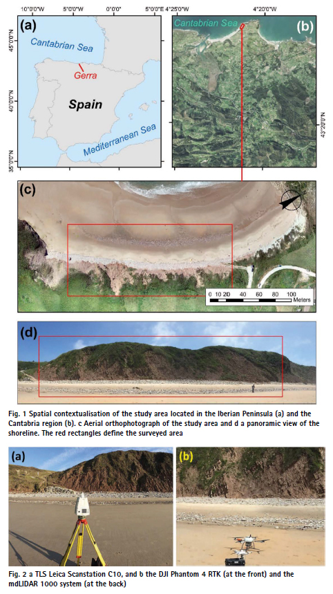
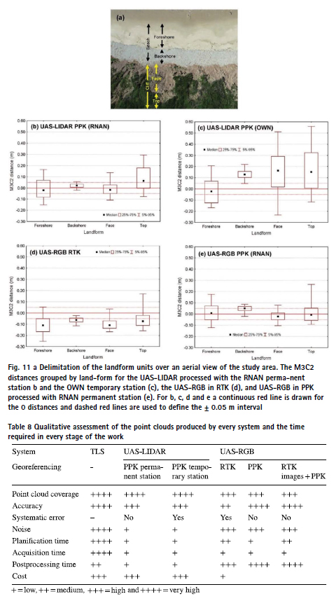
The study was carried out at Gerra beach and cliff (i.e., cliffed coast fronted by a beach with a length of 300 m, from which 200 m were surveyed, Fig. 1), located in a NE-faced small cove in the Cantabria coast, N of Spain (Fig. 1a and b). The climate is temperate oceanic with an average annual rainfall of 1,100 mm distributed along the year and a mean annual temperature of 15° C. The Gerra beach is the easter part of the San Vicente Merón beaches system and may be classified as a composite beach with an unprotected cliff of Eocene sandstones, marls, limestones, and conglomerates to the east and Triassic clays, gypsum and salts to the west. The study area shows four morphological units modelled by different geomorphological processes (Fig. 1c and d). The first two units belong to the composite beach system: the sandy foreshore with a very low slope gradient and the backshore with a relatively higher slope gradient and coarser sediments (cobbles and boulders) supplied by the erosion of the cliff. The third morphological unit is the face of the cliff that joins the beach and the top of the cliff and inland (fourth morphological unit), where we observe “rasas”, i.e. ancient abrasion platform. The top of the cliff has an average altitude of 40 m ASL.
The tidal range is about 4 m so the area is considered a mesotidal environment (de Sanjosé Blasco et al. 2020). The sandy foreshore is modelled by the wave action and nearshore currents. Large storms control backshore dynamics which is continuously supplied of sediments from the cliff due to small rockfalls and landslides. These slope processes on the cliff range in magnitude from 1 to 1000 m3 and are controlled by lithology and structure (folded layers and contact between lithologies) (de Sanjosé Blasco et al. 2020). The recent work by de Sanjosé-Blasco et al. (2020) analysed the dynamics of the area for the period from 1956 to 2020 using several geomatic techniques (classical photogrammetry, SfM-UAS photogrammetry, and TLS) and observed an increase in the cliff retreat rates in the last years, leading to more frequent large magnitude slope processes and unstable cliffs.
Material and methods
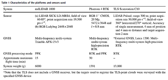
This section describes the instruments, techniques and methods used to perform the analyses. The first four sections describe the acquisition of data by means of the TLS (Fig. 2a), the GNSS, the UAS-LIDAR (Fig. 2b), and the UASRGB (Fig. 2b). The last section details the estimation of distances from every dataset to the benchmark point cloud. All the data was collected simultaneously during low tide. In the analyses, only the overlapping area between all techniques and the stable part of the beach was considered (defined by the red rectangle in Fig. 1); that is, the area affected by the low tide action was not considered.
Terrestrial laser scanner
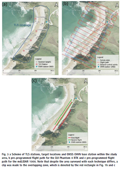
The benchmark model of the study area was obtained using a TLS Leica Scanstation C10 device (Fig. 2a and Table 1). Four stations were planned to minimize the occlusions and cover the surveyed area (Fig. 3a). The registration of the 4 point clouds was carried out by means of nine circular targets model HDS from Leica (with a diameter of 15.24 cm), initially in a relative coordinate system. These targets may be oriented to be registered by any location of the TLS. Additionally, the targets may be set horizontally to survey the geometrical centre of the target in an absolute reference system using a GNSS receiver. From every TLS station, every target is surveyed individually with an accuracy of 2 mm according to TLS manufacturer’s specifications. Figure 3 shows the location of the targets and the stations of the TLS instrument. The registered point cloud is then georeferenced using the absolute coordinates of the targets previously surveyed by the GNSS rover in RTK mode (receiving real-time corrections from the OWN station, see the Sect. “Global navigation satellite systems”). The geo-referencing error of this point cloud was 0.8 cm.
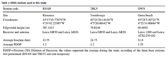
Global navigation satellite systems
Three GNSS stations were used for the post-processing of the UAS trajectories. The first was an own station stablished temporarily within the study area (named “OWN” ahead, with an average baseline of 0.14 km, Table 2). The second and third are permanent GNSS stations that belong to the regional Cantabrian continuously operating reference stations (CORS) network. Specifically, Rionansa (RNAN) and Torrelavega (TRLV) stations, located at 13 and 25 km from the study area, respectively. The range of distances (from 0.14 to 25 km) allows to explore the role of the baseline in the final accuracy obtained. The coordinates of the OWN station were calculated by using static records longer than 1 h and simultaneous data registered at 1 s temporal resolution at RNAN and TRLV. Additionally, the OWN station was used to send corrections in real-time to a mobile receiver (Fig. 1b) operating in the study area to survey the GCPs, the CPs and to georeference the TLS model (surveying the targets). A total of 25 points were surveyed as GCPs (or CPs, see Sect. “UAS-RGB and SfM photogrammetry (RTK, PPK and GCP-based)”) and 9 as TLS targets (Table 3). These GCPs were distributed in the safe area as the top of the cliff is inaccessible for safety reasons.
UAS LIDAR
The mdLIDAR 1000 system by microdrones is a UAS-based LIDAR system (Sick; Fig. 2b) integrated with a camera (to colour the LIDAR-derived point cloud) and a survey grade GNSS (Applanix APX-15 GNSS/IMU) receiver for direct geo-referencing. The LIDAR system has a field of view of 60° or 85°, with 3 returns and an acquisition rate, for both field of views, of 19,500 pts·s−1. The mdLIDAR 1000 has a minimum and maximum flight altitude of 30 m and 50 m, respectively.
The GNSS/IMU system records sensor location and orientation to be postprocessed, i.e., works in PPK mode. The system has 336 channels including GPS (L1 C/A, L2C, L2E, L5), GLONASS (L1 C/A, L2 C/A, L3 CDMA), BeiDou (B1 and B2), Galileo (E1, E5A, E5B, E5Altboc), QZSS (L1 C/A, L1S, L1C, L2C, L5, LEX), SBAS (L1 C/A, L5) and MSS L-band (Trimble RTX, OmniSTAR). The IMU is a Micro Electro Mechanical System-based inertial sensor with a data rate of 200 Hz. The PPK was car-ried out using the POSPac UAS (v. 8.4) (ApplanixTRIMBLE 2022) software and using as input the trajectory file of the UAS (GNSS location and IMU data), the RINEX files of the GNSS permanent stations (Table 2) and the offset parameters between the LIDAR and the GNSS-IMU systems (boresight angles, mounting angles and lever arms). The bore-sight angles, mounting angles and lever arms values are provided directly by the manufacturer in a calibration report specific to each LIDAR-GNSS-IMU unit. The corrected trajectory of the UAS is then used to compute the location of LIDAR 3D points in the mdLIDAR processing software (v. 1.3.0) (MICRODRONES 2022).
Two flights with flight lines parallel to the shoreline were designed to cover the study area (Fig. 3c) and minimize occlusions. The first one at 30 m of altitude above the top of the cliff to monitor, particularly, the upper part of the cliff, but also the rest of the study area with a field of view of 60°. The second one at 50 m of altitude above the beach to monitor the face of the cliff and the beach with a field of view of 85° (Fig. 3c). Both flights were designed using the mdcockpit app running in a tablet (Samsung S5 with android operative system) and the same app was used at field to monitor data acquisition and UAS telemetry. The whole data acquisition was carried out autonomously according to the predefined flight plan. Flights 1 and 2 had a total duration of 5′24″ and 4′57″ respectively, both flights were carried out at a speed of 3 m·s−1. During each flight, the UAS automatically performs two manoeuvres, at the beginning and at the end, necessary for calibrating the IMU. According to the manufacturer the integrated system has an absolute vertical and horizontal accuracy of ± 6 cm. The potential misalignment between the two UAS-LIDAR flights was analysed by selecting the overlap area and calculating the distances between the two point clouds in this area. The calculation of the distance between point clouds was based on the Multiscale Model-to-Model Cloud Comparison algorithm (M3C2: Lague et al. 2013. See Sect. “Analysis of the resulting point clouds”). No misalignment was observed between the flights in the overlap zone, so the two flights were merged without any co-registration procedure. The UAS trajectories were processed using the three GNSS stations independently, and the best solution was selected for subsequent analyses (M3C2 distances to the benchmark TLS model).
UAS-RGB and SfM photogrammetry (RTK, PPK and GCP-based)
The DJI Phantom 4 RTK is a multirotor with a multi-frequency GNSS system and a built-in 1″ RGB CMOS sensor with 20 Mpx on board (Fig. 2b and Table 1). The GNSS system receives and records GPS L1/L2, GLONASS L1/ L2, BeiDou B1/B2 and Galileo E1/E5. The RGB sensor has a lens with a field of view of 84° and a focal length of 8.8 mm (35 mm for-mat equivalent: 24 mm).
Three datasets were produced by means of the UAS-RGB and the SfM photogrammetry. The first one was fed by images acquired receiving RTK corrections via NTRIP (Networked Transport of RTCM via Internet Protocol) from a 4G internet connection to the regional (Cantabrian) GNSS service of real-time corrections (network solution NTRIP protocol in format RTCM3.1, MAC3). This dataset will be named ahead UAS-RGB RTK. The second dataset was produced using the same images of the dataset one but post-processed using a PPK approach by means of the REDcatch-REDtoolbox software (REDcatch 2022) that performs the position correction of the UAS at every photo acquisition using the permanent stations data recorded simultaneously. This information is recorded in the EXIF file of the images and used in the photogrammetric processing to constrain camera location and position uncertainty. This dataset will be named UAS-RGB RTK images+PPK and consists of a PPK approach using the same images of the RTK approach. The third approach used the same flight plan of the former two datasets (Fig. 3b) to acquire images just recording data without real time corrections to carry out a PPK approach later (UAS-RGB PPK). The comparison between datasets will allow to analyse the effect of postprocessing type and changes in image acquisition conditions (such as lighting) on the final accuracy of the results.
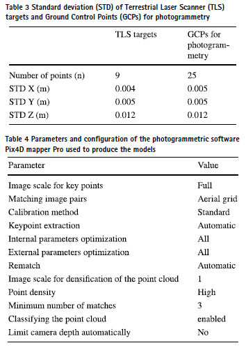
The flights were planned at an altitude of 80 masl, resulting in an average GSD of 2.19 cm and following the track shown in Fig. 3b. The front and side overlap were set to 80% and flight speed was the maximum allowed for this configuration (6.3 m·s−1 ). The flight time was approximately 11 min. The camera was close to nadir with a deviation of 4° from nadir. The images obtained by every workflow, the RTK, the RTK + PPK and the PPK, were used as input in the photogrammetric software, in this case Pix4D-mapper Pro (v.4.5.6) (PIX4D-SA 2022). A total of 282 images were acquired during each flight with a resolution of 5,472·3,648 pixels. The points recorded by the rover GNSS device were marked in all the images and used to estimate the Root Mean Square Error (RMSE) in models with a varying number of CPs and GCPs. The 25 surveyed points were used as CPs in the models without GCPs (i.e., GCP = 0) but additionally, we explored the role of an increasing number of GCPs in the final accuracy of the resulting models. To do this, we used one GCP to support the model and the rest as CPs. The procedure was repeated using every point as GCP and the rest as CPs and the average RMSE was calculated. Then, the procedure was repeated using 2, 3,.., 25 GCPs, and calculating the average RMSE. For example, for 3 GCPs all possible combinations of 3 GCP were used and the remaining 22 points were used as CPs to calculate the average RMSE.
For models without GCPs, the influence of the altitude optimization was explored. This option was introduced at the end of 2019 by DJI manufactures to minimize the wrong absolute altitude estimation in surveys without GCPs. A set of oblique images, in addition to the nadiral ones, are collected if this option is set. We processed the datasets with and without this set of oblique images and compared the accuracy of the resulting models. The photogrammetric processing within the Pix4Dmapper Pro software was carried out with the configuration shown in Table 4.
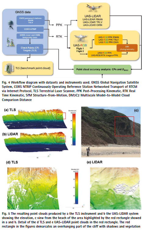
Analysis of the resulting point clouds
he resulting point clouds were characterized and analysed in terms of point density and coverage. Volumetric point density was calculated using a sphere with radius 0.62 m, which results in a volume of 1 m3 . Additionally, the algorithm M3C2 (Lague et al. 2013) was used to estimate the distance between the benchmark point cloud acquired by the TLS and the SfM (RTK or PPK) or LIDAR-derived point clouds (ahead DM3C2) (Fig. 4). The M3C2 algorithm is a change detection method for point clouds that calculates 3D distances and uncertainties. First, the algorithm estimates local surface normal (N) by fitting a plane to points in cloud 1 within a neighbourhood defined by a parameter named normal scale (D). The N determines the direction in which changes will be measured. Then, a cylinder, with radius d (projection scale) and height h is projected from point cloud 1 to point cloud 2 along the N vector. Finally, the average positions of points within the cylinder in each cloud are calculated, and the distance between these positions along the N is the DM3C2. The suitable values for D and d were empirically evaluated, and those that resulted in N values that best represented the landforms in the study area were used. The resulting DM3C2 shows the absolute agreement of the analysed point cloud regarding the benchmark model due to all the components of error. In this analysis, the two compared point clouds were acquired simultaneously so we did not use the uncertainty estimation of DM3C2 and every calculated value is considered as error. The statistical analysis of the DM3C2 variability, using the standard deviation of the DM3C2, for instance, may also provide insight into the range of errors (Nesbit et al. 2022). This analysis was carried out for two datasets acquired by the UAS-RGB RTK (the RTK NTRIP and the most accurate PPK) and the one acquired by the UAS-LIDAR (the PPK dataset with the OWN and RNAN GNSS stations). The preparation of the point clouds and the estimation of the DM3C2 was carried out in CloudCompare software (v. 2.12.0) (GPL-Software 2022).
Results
TLS point cloud
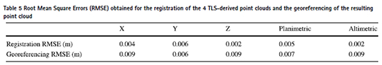
The benchmark TLS-derived point cloud showed a total of 23.4 million of points, with an average point density of 41,156 pts·m−3 (Fig. 5). The TLS coverage was homogeneous, except for small, highly intricate areas in the western part of the cliff (right of the Fig. 5a). The TLS model benefited from the ground perspective, getting points in a shaded and overhanging part of the cliff partially covered by vegetation (Fig. 5d). Table 5 shows the registration and the geo-referencing RMSEs for the TLS dataset. The registration based on targets showed errors lower than 0.006 m while the geo-referencing, based on the coordinates of the targets surveyed by the GNSS in RTK mode, increased errors from 0.005 to 0.007 m and 0.002 to 0.009 m for the planimetric and altimetric components, respectively.
UAS-LIDAR point cloud
The UAS-LIDAR-derived point cloud showed a point density of 27,293 pts·m−3 . The resulting LIDAR-derived point cloud has a large coverage (Fig. 5b), being the only aerial technique tested here that captured points in specific overhanging parts of the cliff (Fig. 5e). It was estimated, during post-processing in the Pospac software, a 3D RMSE of 0.035 m for the RNAN solution. The PPK processing using different permanent stations produced slight differences in the RMSEs, indicating that, as expected, GNSS stations with baselines < 25 km result in highly accurate point clouds. Three-dimensional RMSEs of 0.037 m and 0.039 m were estimated for TRLV and OWN solutions. From this point on and in subsequent analyses, for the LIDAR data, those obtained using the permanent RNAN station and the temporary OWN station will be used.
UAS-RGB point clouds
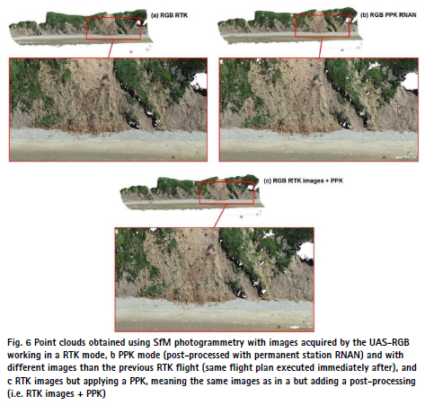
The point clouds produced using the UAS-RGB and the SfM photogrammetry technique showed point densities that varied from 964 to 1,163 pts·m−3 (Fig. 6). The images used to produce the point clouds in the RTK and the PPK modes were acquired during different flights, consequently, point density for both datasets were slightly different. The point clouds produced with the same images but with different processing methods (RTK vs RTK images + PPK) showed significant differences regarding the presence of data gaps. In fact, the point clouds generated with PPK and RTK images + PPK processing were very similar despite being produced using images acquired in different flights (Fig. 6b and c), indicating that certain processing factors have a decisive influence on the existence of data gaps in the final point cloud. The SfM-derived point clouds showed gaps in the overhanging area and at some vegetated sites over the face and top of the cliff (Fig. 6).
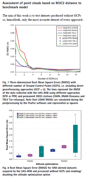
According to the RMSE (Fig. 7), the PPK workflow, independently of the GNSS permanent station used, resulted in more accurate models than the RTK approach. The models obtained in PPK with the RNAN GNSS station were the most accurate in the absence of GCPs (Fig. 7). Our OWN GNSS station did not resulted in the most accurate models despite being the closest one, with an average baseline of 0.14 km. The OWN station also showed the larger Position Dilution of Precision (PDOP = 1.53) compared to RNAN or TRLV (PDOP = 1.20).
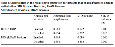
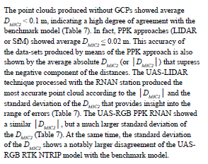
Figure 7 shows that the addition of GCPs slightly increased the accuracy of the UAS-RGB resulting models. The RTK approach was particularly benefited by the inclusion of up to 3 GCPs. From 3 GCPs upwards, improvements in the accuracy of the resulting models were negligible. In the PPK approach the influence of adding GCPs was very slight. We did not observe any significant enhancement of adding GCPs to the PPK RNAN dataset (Fig. 8). The altitude optimization option in the UAS-RGB datasets played a crucial role to reduce the errors in the final models, particularly in the absolute altitude estimation (Fig. 8). The models produced using the oblique photographs acquired due to the altitude optimization option (in PPK or RTK) resulted in more accurate estimations of the camera focal length than those produced using only the nadiral photographs (Table 6). The RTK approach was the most benefited of enabling the altitude optimization option (Table 6). In the RTK approach, the Z coordinate RMSE improved from 0.37 m to 0.12 m when the oblique photographs were used. The X and Y RMSEs of the PPK datasets were also reduced with the use of the oblique photographs. Specifically, the RMSE for the X coordinate decreased from 0.06 to 0.04 m, while the Y-RMSE lessened from 0.09 to 0.04 m.
Assessment of point clouds based on M3C2 distance to benchmark model
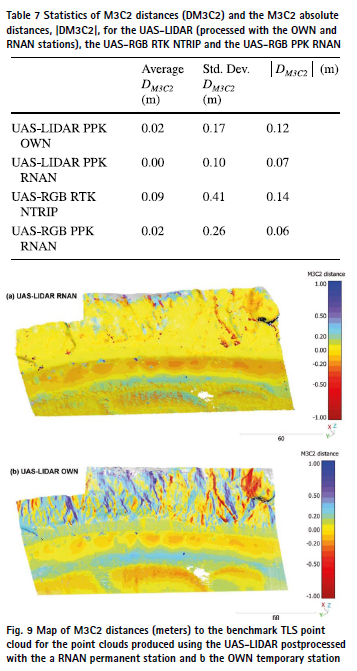
The aim of this work is to test datasets produced without GCPs so, henceforth, only the most accurate dataset of every approach and technique will be used in the upcoming analysis: the UASLIDAR RNAN (permanent station), the UAS-LIDAR PPK OWN (temporary station), the UAS-RGB RTK NTRIP, the UAS-RGB PPK RNAN and the UAS-RGB RTK images processed with PPK. In the case of the SfM-derived datasets, they were acquired setting the altitude optimization option. Furthermore, the LIDAR and photogrammetric systems have such different characteristics (e.g. flight altitude, overlap, etc.) that comparing them would not be fair. However, we can extract valuable information by comparing the RTK and PPK approaches in the case of photogrammetry or the analysis of the accuracies for each landform.
The maps of DM3C2 show significant differences between techniques and approaches (Fig. 9 and Fig. 10). LIDAR point clouds processed using the RNAN permanent station solution revealed significantly lower DM3C2 values compared to those processed with the OWN temporary station (Fig. 9). The differences were particularly noticeable on the cliff face and the backshore. The LIDAR data exhibited minimal noise, with only a few noisy points observed in the foreshore. The photogrammetric point clouds showed noise in the front of the foreshore with the noise decreasing inland (Fig. 10). The postprocessed photogrammetric clouds presented significantly lower errors compared to the RTK point cloud. The noise and instrumental errors for every point cloud are reflected in the length of the 5–95% interval in Fig. 11, while the distance from the median to the DM3C2 = 0 shows the bias of the dataset (systematic error), related to the geo-referencing approach (also in Fig. 11). The datasets post-processed with the RNAN station solution did not exhibit systematic errors (UAS-LIDAR and UAS-RGB PPK; Fig. 11) indicating that these datasets can be used without any prior co-registration procedure to be compared to other cartographic products. The UAS-RGB RTK showed a negative bias while the UAS-LIDAR post-processed with the OWN temporary station solution presented a positive bias in the backshore, the face, and the top of the cliff. The analysis of DM3C2 disaggregated by landform and technique provided insight about the achievable accuracy of the geo-referencing without GCPs approach in these environments under similar flight and instruments conditions. If we focus on the datasets post-processed with the RNAN permanent station that do not show systematic errors, we can observe that the 5–95% interval width is substantially larger for the foreshore and top of the cliff landforms compare to the backshore and the face of the cliff.
Discussion
The laser-based techniques resulted in dense point clouds with homogeneous coverage, specifically the UAS-LIDAR system acquired points in vegetated overhanging parts of the cliff (Fig. 5). Table 8 shows a qualitative assessment of the characteristics of each point cloud along with the processing time required for each phase of its production and cost of the equipment. The SfMderived point clouds showed data gaps in an overhanging part in the face of the cliff, some vegetated spots, and some parts of the foreshore beach. We found differences in the distribution of data gaps in the point clouds produced with the same images but different processing methods (e.g., RTK vs RTK images + PPK). However, the pattern of data gaps was similar for point clouds generated with the PPK and the RTK images + PPK approaches despite using different images in each procedure (acquired with the same flight plan). The RTK approach minimizes data gaps compared to the PPK and the RTK images+PPK approaches (Fig. 6), which would indicate that by exhibiting lower accuracy in the positioning of each camera, it would provide more freedom to the photogrammetric processing. The reduction in the positional accuracy of the images may influence: (a) the overlap between images that may be seemingly greater with more information available for the 3D reconstruction, (b) the number of matches or correspondences between visual features in the images leading to a greater number of detected key points and, (c) the uncertainty in the estimation of the position of each point in the cloud which will be larger, resulting in more redundant or erroneous points, contributing to a higher apparent density in the point cloud. This finding is an interesting element to explore in future research as the point cloud generated with RTK processing could be used to fill data gaps in a point cloud generated with PPK processing that according to our results shows a higher accuracy.
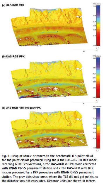
Data gaps in overhanging parts are typical in UAS-derived point clouds using SfM photogrammetry and nadir acquisition angles (Jaud et al. 2019). Jaud et al. (2019) suggested the use of higher tilting angles to reduce data gaps in these vertical or over-hanging parts of the cliff and Gómez-Gutiérrez and Gonçalves (2020) directly acquired UAS off-nadir images to model almost vertical coastal cliffs. To deal with these data gaps, in projects interested in the dynamics of the coastline (considering the beach and the top of the cliff) alternatives may be the combination of aerial and terrestrial techniques (Ismail et al. 2022) or the use of varying tilting angles (Jaud et al. 2019). Vegetated surfaces are one of the biggest limitations for SfM-derived 3D models (Westoby et al. 2012; Gomez-Gutierrez et al. 2014). Our study shows a good performance of the UAS-LIDAR (Fig. 5) to overcome the limitations of coastal cliffs (overhanging areas and image poor texture in vegetated or sandy surfaces). The decrease in prices of UAS-LIDAR systems in the last years is positioning this technology as an important alternative to photogrammetry (Pereira et al. 2021; Štroner et al. 2021a, b), particularly for vegetated (or partially vegetated) and complex surfaces like the Gerra study area. Data gaps and noise observed in the foreshore beach for SfM photogrammetry (Fig. 10) are considered a consequence of images’ texture in this place while the data gap observed in the foreshore beach for the UAS-LIDAR dataset correspond to a thin water pool (Fig. 9). The presence of noise and vegetation gaps in the photogrammetric point clouds results in a wide range of the DM3C2 as can be observed in Fig. 11c and d for the foreshore and the top of the cliff. Note that the range of DM3C2 is independent of the geo-referencing systematic error, being the latter represented by an offset between the median DM3C2 and 0 in Fig. 11. For example, the UAS-LIDAR OWN in the backshore shows high precision with a short range of DM3C2 but, at the same time, an offset for the median DM3C2 that should be handled with a co-registration procedure if the user is interested on the comparison with other cartographic products.
The geo-referencing methods without GCPs based on the PPK approach outperformed the RTK approach in terms of accuracy, with the resulting RTK accuracy observed being similar to the few previous experiences (Hugenholtz et al. 2016; Eker et al. 2021;). The out performance of PPK over RTK approach has to do with several factors: (i) the availability of precise ephemeris data of satellites for the post-processing, providing a more accurate solution (Zhang et al. 2019), (ii) the absence of latency for the application of corrections (Puente et al. 2013) and (iii) the limitation of communication and linkage problems between the rover and the corrections’ provider. Despite these advantages, the PPK resulting accuracy is unknown beforehand, relying on the continuous record of data by a nearby GNSS base station. The selection of the GNSS base station is crucial in the case of UASLIDAR with the permanent stations providing a solution that resulted in a point cloud free from systematic errors, in contrast to the temporary station that exhibited this error. This finding is particularly relevant for the monitoring of remote and hard-to-reach areas (Elias et al. 2024), where permanent stations are typically not available, making it necessary to use a temporary base station. In our case, the temporary OWN station was located on a concrete path that provides access to the beach, i.e. on a stable surface not exposed to the effects of tides, and potential rockfalls or landslides. In terms of coverage, the ideal location for this station would be the top of the cliff, although this area is not without risks and the philosophy of this work was to carry out the monitoring of inaccessible or dangerous landforms at the minimum risk. Regarding the influence of the baseline length for the PPK approaches, we did not find any significant difference for the two permanent stations with baselines < 25 km and PDOP < 2.5 (Puente et al. 2013), neither the SfM photogrammetry nor the UAS-LIDAR, similarly to the findings of the previous works by Dreier et al. (2021) or Eker et al. (2021).
The errors estimated during the processing of the trajectory of the UASLIDAR dataset (3D RMSE of 3.5 cm for RNAN station), and the calculated DM3C2 and │DM3C2 │ (Table 7) agreed in magnitude with previous studies (Gallay et al. 2016; Glennie et al. 2016; Salach et al. 2018) and with manufacturer’s specifications (6 cm). These figures add insight to the scarce literature about the accuracy of UAS-LIDAR instruments (Mayr et al. 2020). Focusing exclusively on positional accuracy, the analysis showed that the UAS-LIDAR RNAN produced the best point cloud, followed by the UAS-RGB PPK RNAN, which exhibited a similar │DM3C2 │but a larger standard deviation of the DM3C2 , due to a greater presence of noise in the point cloud. The point clouds obtained from the post-processing with RNAN data were the only ones that did not exhibit systematic errors, indicating that they could be compared with other cartographic products without the need of any prior co-registration procedure. However, in all other cases, including data acquisition using RTK, this co-registration would be necessary prior to comparison. Some recent studies have managed to increase the positional accuracy of data generated with UAS-LIDAR (from cm to mm) through hybrid geo-referencing supported by photogrammetric data acquired simultaneously (Haala et al. 2022). However, these strategies still require the presence of GCPs or control planes.
The differences observed in the DM3C2 for the various landforms are substantial and allow us to tune future topographic change analyses using spatially distributed thresholds (Lague et al. 2013; James et al. 2017a, b; Mayr et al. 2020; Winiwarter et al. 2021; Zahs et al. 2022). In both the UAS-LIDAR RNAN and UAS-RGB PPK RNAN data, we have observed that in the backshore and cliff face, the threshold for distinguishing topographic change from noise can be reduced compared to the foreshore and the top of the cliff. In the case of the LIDAR, the beach may feature small water ponds, while at the top of the cliff, the presence of vegetation also affects the positional accuracy of LIDAR data, as has been observed with airborne sensors (Mayr et al. 2020). In the case of UAS-RGB PPK RNAN, the previous mentioned factors related to poor image texture (vegetation, sand, and water) are the underlying causes of these differences.
The systematic bias in the absolute altitude found in the recent literature for SfM-models produced using georeferencing approaches without GCPs (e.g. Liu et al. 2022; Taddia et al. 2020a, b) is completely removed in the PPK (Fig. 11e) and substantially reduced in the RTK approach using the oblique photographs acquired by enabling the altitude optimization option within the DJI GS RTK app (Fig. 8). However, if the final purpose of these models is the estimation of topographic changes, the reduced bias may still produce significant over or under-estimations in the case of the RTK approach (Fig. 11c). In this case, we found that the use of three GCPs (similarly to Liu et al. 2022) (Fig. 8) or a previous co-registration of the models would be necessary to produce the most accurate estimations. Recent studies have shown an interesting alternative to traditional co-registration strategies (i.e. the use of the Iterative Closest Point algorithm in stable areas), based on the simultaneous processing of multitemporal images (Feurer and Vinatier 2018; Blanch et al. 2021), but, to our knowledge, this approach has not been tested yet on RTK or PPK datasets.
The Table 8 shows a qualitative assessment of the point clouds generated by the instruments and techniques used, which can be useful for researchers looking to select the appropriate technique for a specific task. In summary, the TLS offers dense point cloud coverage and accuracy but requires long planning, acquisition and postprocessing time and comes at a high cost. The UAS-LIDAR provides high point cloud coverage and precision with short planning and postprocessing times. The selection of the GNSS base station for postprocessing the UAS-LIDAR data must be done with care. In our case, the permanent station RNAN produced an accurate point cloud free from systematic errors. However, the point cloud post-processed with the temporary OWN station exhibited systematic error, making it necessary to co-register this data before comparing it with any other spatial data. The UAS-RGB system in RTK shows moderate accuracy, with noise and systematic errors present. Finally, the UAS-RGB with PPK approaches were the most cost-effective with high accuracy and without systematic errors, however, there are likely to be gaps in densely vegetated areas as well as noise in areas with poor image texture.
Conclusions
We produced point clouds of the coastline by means of two UAS with different sensors (the UAS-LIDAR and the UAS-RGB) without the need of GCPs and compared the results with a benchmark model surveyed with a TLS device. This benchmark model produced a very accurate point cloud with the highest coverage but required long planning, acquisition and postprocessing time and comes at high cost.
The UAS-LIDAR, that only works in PPK, produced a point cloud without noise, with a homogeneous coverage, with low planning and postprocessing time. For this platform-sensor we have observed that the selection of the station used to correct the UAS trajectory is crucial. The use of a nearby permanent station resulted in a point cloud free of systematic error, whereas the use of a temporary station located in the study area produced a point cloud with some degree of systematic bias. According to our results the UAS-LIDAR processed with the RNAN permanent station produced the most accurate point cloud. The UAS-RGB performing in RTK resulted in point clouds with systematic errors in the foreshore, the face and top of the cliff. This bias was substantially reduced using the oblique images acquired by enabling the altitude optimization option and completely removed in the PPK approach. Both photogrammetric pipelines (RTK and PPK) showed other limitations: data gaps in vegetated areas, noise in the foreshore and long postprocessing times. Hence, the UAS-RGB with PPK was the most cost-effective method however the advantages of the UAS-LIDAR (accuracy, low noise, homogeneous and dense coverage) along with the decrease in the prices of UAS-LIDAR systems make it an interesting alternative.
Acknowledgements
The authors would like to express their gratitude to the three anonymous reviewers who contributed to improve the quality of this manuscript. This work was funded by: (1) the Junta de Extremadura and FEDER (Grant numbers: GR21154 and GR21156), (2) The Spanish Ministry of Economy and Competitiveness (Grant number: UNEX13-1E-1549), (3) the Spanish Agency of Research (Grant number: EQC2018-004169-P) and (4) Grant PID2022-137004OB-I00 funded by MCIN/ AEI/https:// doi. org/ 10. 13039/ 50110 00110 33 and by “ERDF A way of making Europe”, by the “European Union”. These sponsors have not played any role in the design and development of the study.
Authors contributions
All authors contributed to the study conception and design. Material preparation, data collection and analysis were performed by AGG, JJB and MSF. The first draft of the manuscript was written by AGG and all authors commented on previous versions of the manuscript. Reviews were carried out by AGG and MSF. All authors read and approved the final manuscript. Funding Open Access funding provided thanks to the CRUE-CSIC agreement with Springer Nature. This work was funded by: (1) the Junta de Extremadura and FEDER (Grant numbers: GR21154 and GR21156), (2) The Spanish Ministry of Economy and Competitiveness (Grant number: UNEX13-1E-1549), (3) the Spanish Agency of Research (Grant number: EQC2018-004169-P) and (4) GrantPID2022-137004OB-I00 funded by MCIN/AEI/https://doi. org/10.13039/501100011033 and by “ERDF A way of making Europe”, by the “European Union”. These sponsors have not played any role in the design and development of the study.
Data availability The datasets generated during and/or analysed during the current study are available from the corresponding author on reasonable request.
Declarations
Competing interests The authors declare no competing interests.
Open Access This article is licensed under a Creative Commons Attribution 4.0 International License, which permits use, sharing, adaptation, distribution and reproduction in any medium or format, as long as you give appropriate credit to the original author(s) and the source, provide a link to the Creative Commons licence, and indicate if changes were made. The images or other third party material in this article are included in the article’s Creative Commons licence, unless indicated otherwise in a credit line to the material. If material is not included in the article’s Creative Commons licence and your intended use is not permitted by statutory regulation or exceeds the permitted use, you will need to obtain permission directly from the copyright holder. To view a copy of this licence, visit http:// creativecommons.org/licenses/by/4.0/.
References
Ahokas E, Kaartinen H, Hyyppä J (2003)
A quality assessment of airborne laser scanner data. Int Arch Photogramm Remote Sens Spatial Inform Sci 34:1–7
Applanix-TRIMBLE (2022) PosPac UAV
Baltsavias EP (1999) Airborne laser scanning: basic relations and formulas. ISPRS J Photogramm Remote Sens 54(2):199–214
Benassi F, Dall Asta E, Diotri F, Forlani G, Morra di Cella U, Roncella R, Santise M (2017) Testing accuracy and repeatability of UAV blocks oriented with GNSS-supported aerial triangulation. Remote Sens 9(2):172
Besl PJ, McKay ND (1992) A Method for Registration of 3-D Shapes. IEEE Trans Pattern Anal Mach Intell 14(2):239–256
Blanch X, Eltner A, Guinau M, Abellan A (2021) Multi-epoch and multi-imagery (MEMI) photogrammetric workflow for enhanced change detection using time-lapse cameras. Remote Sens 13(8):1460
Carbonneau PE, Dietrich JT (2017) Cost-effective non-metric photogrammetry from consumer-grade sUAS: implications for direct geo-referencing of structure from motion photogrammetry. Earth Surf Proc Land 42(3):473–486
Colomina I, Molina P (2014) Unmanned aerial systems for photogrammetry and remote sensing: a review. ISPRS J Photogramm Remote Sens 92:79–97
Cramer M, Stallmann D, Haala N (2001) Direct geo-referencing using GPS/inertial exterior orientations for photogrammetric applications. Int Arch Photogramm Remote Sens 33:198
Cramer M, Haala N, Laupheimer D, Mandlburger G, Havel P (2018) Ultra-high precision uavbased lidar and dense image matching. Int Arch Photogramm Remote Sens Spatial Inf Sci XLII–1:115–120
Darmawan H, Walter TR, Brotopuspito KS (2018) Morphological and structural changes at the Merapi lava dome monitored in 2012–15 using unmanned aerial vehicles (UAVs). J Volcanol Geoth Res 349:256–267
de Sanjosé Blasco JJ, Serrano-Cañadas E, SánchezFernández M, Gómez-Lende M, Redweik P (2020) Application of multiple geomatic techniques for coastline retreat analysis: the case of Gerra Beach (Cantabrian Coast, Spain). Remote Sens 12(21):3669
Del Río L, Gracia FJ (2009) Erosion risk assessment of active coastal cliffs in temperate environments. Geomorphology 112(1):82–95
Dreier A, Janßen J, Kuhlmann H, Klingbeil L (2021) Quality analysis of direct geo-referencing in aspects of absolute accuracy and precision for a UAV-based laser scanning system. Remote Sens 13(18):3564
Eker R, Alkan E, Aydin A (2021) Accuracy comparison of UAV-RTK and UAV-PPK methods in mapping different surface types. Eur J Forest Eng. https:// doi. org/ 10. 33904/ ejfe. 938067
Elias M, Isfort S, Eltner A, Mass HG (2024) UAS Photogrammetry for precise digital elevation models of complex topography: a strategy guide. ISPRS Ann Photogramm Remote Sens Spatial Inf Sci X–2:57–64
Eltner A, Sofia G (2020) Structure from motion photogrammetric technique. Remote Sens Geomorphol. https:// doi. org/ 10. 1016/ b978-0- 444- 64177-9. 00001-1
Emery KO, Kuhn GG (1982) Sea cliffs: their processes, profiles, and classification. Geol Soc Am Bull 93(7):644–654 Feurer D, Vinatier F (2018) Joining multi-epoch archival aerial images in a single SfM block allows 3-D change detection with almost exclusively image information. ISPRS J Photogramm Remote Sens 146:495–506
Forlani G, Dall’Asta E, Diotri F, Cella UMD, Roncella R, Santise M (2018) Quality assessment of DSMs produced from UAV flights georeferenced with on-board RTK position-ing. Remote Sens 10(2):311
Gallay M, Eck C, Zgraggen C, Kaňuk J, Dvorný E (2016) High resolution airborne laser scanning and hyperspectral imaging with a small uav platform. Int Arch Photogramm Remote Sens Spatial Inf Sci. XLI-B1:823–827
CLGlennie A Kusari A Facchin 2016 Calibration and stability analysis of the vlp-16 laser scanner Int Arch Photogramm Remote Sens Spatial Inf Sci10.5194/ isprs-archives-XL-3-W4-55-2016Glennie CL, Kusari A, Facchin A (2016) Calibration and stability analysis of the vlp-16 laser scanner. Int Arch Photogramm Remote Sens Spatial Inf Sci. https://doi. org/ 10. 5194/ isprs-archi ves- XL-3- W4- 55- 2016
Gomez-Gutierrez A, Schnabel S, Berenguer-Sempere F, Lavado-Contador F, Rubio-Delgado J (2014) Using 3D photo-reconstruction methods to estimate gully headcut erosion. CATENA 120:91
Gómez-Gutiérrez A, Goncalves GR (2020) Surveying coastal cliffs using two UAV platforms (multirotor and fixed-wing) and three different approaches for the estimation of volumetric changes. Int J Remote Sens 41(21):8143–8175
Goulden T, Hopkinson C (2010) The forward propagation of integrated system component errors within airborne lidar data. Photogramm Eng Remote Sens 76(5):589–601
GPL-Software (2022) CloudCompare
Haala N, Kölle M, Cramer M, Laupheimer D, Zimmermann F (2022) Hybrid geo-referencing of images and LIDAR data for UAV-based point cloud collection at millimetre accuracy. ISPRS Open J Photogramm Remote Sens 4:100014
Heipke C, Jacobsen K, Wegmann H, Nilsen B (2001) Integrated sensor orientation—An Oeepe Test. 33
Hodgson M, Bresnahan P (2004) Accuracy of airborne LIDARderived elevation: empirical assessment and error budget. Photogramm Eng Remote Sens 70:331–339
Hugenholtz C, Brown O, Walker J, Barchyn T, Nesbit P, Kucharczyk M, Myshak S (2016) Spatial accuracy of UAV-derived orthoimagery and topography: comparing photogrammetric models processed with direct geo-referencing and ground control points. Geomatica 70:21–30
Ismail A, Ahmad Safuan AR, Sa’ari R, Wahid Rasib A, Mustaffar M, Asnida Abdullah R, Kassim A, Mohd Yusof N, Abd Rahaman N, Kalatehjari R (2022) Application of combined terrestrial laser scanning and unmanned aerial vehicle digital photogrammetry method in high rock slope stability analysis: a case study. Measurement 195:111161
James MR, Robson S (2014) Mitigating systematic error in topographic models derived from UAV and ground-based image networks. Earth Surf Proc Land 39(10):1413–1420
James MR, Robson S, D’Oleire-Oltmanns S, Niethammer U (2017a) Optimising UAV topographic surveys processed with structure-frommotion: ground control quality, quantity and bundle adjustment. Geomorphology 280:51–66
James MR, Robson S, Smith MW (2017b) 3-D uncertainty based topographic change detection with structure-frommotion photogrammetry: precision maps for ground control and directly georeferenced surveys. Earth Surf Proc Land. https:// doi. org/ 10. 1002/ esp. 4125
Jaud M, Letortu P, Théry C, Grandjean P, Costa S, Maquaire O, Davidson R, Le Dantec N (2019) UAV survey of a coastal cliff face—selection of the best imaging angle. Measurement 139:10–20
GJóźków CTothD Grejner‑Brzezinska 2016 UAS topographic mapping with velodyne LiDAR sensorISPRS Annal Photogramm Remote Sens Spat Inform Sci10.5194/ isprsannals-III-1-201- 2016Jóźków G, Toth C, Grejner-Brzezinska D (2016) UAS topographic mapping with velodyne LiDAR sensor. ISPRS Annal Photogramm Remote Sens Spat Inform Sci. https:// doi. org/ 10. 5194/ isprs annals- III-1- 201- 2016
Lague D, Brodu N, Leroux J (2013) Accurate 3D comparison of complex topography with terrestrial laser scanner: application to the Rangitikei canyon (N-Z). ISPRS J Photogramm Remote Sens 82:10–26
Liu X, Lian X, Yang W, Wang F, Han Y, Zhang Y (2022) Accuracy assessment of a UAV direct geo-referencing method and impact of the configuration of ground control points. Drones 6(2):30
AMayrMBremerMRutzinger20203D point errors and change detection accuracy of unmanned aerial vehicle laser scanning dataISPRS Ann Photogramm Remote Sens Spatial Inf Sci10.5194/ isprs-annals-V-2-2020-765-2020Mayr A, Bremer M, Rutzinger M (2020) 3D point errors and change detection accuracy of unmanned aerial vehicle laser scanning data. ISPRS Ann Photogramm Remote Sens Spatial Inf Sci. https:// doi. org/ 10. 5194/isprs- annals- V-2- 2020- 765- 2020
OMian JLutes GLipaJJHutton EGavelle SBorghini 2016 Accuracy assessment of direct geo-referencing for photogrammetric applications on small unmanned aerial platformsInt Arch Photogramm Remote Sens Spatial Inf Sci10.5194/ isprsarchives-XL-3-W4-77-2016Mian O, Lutes J, Lipa G, Hutton JJ, Gavelle E, Borghini S (2016) Accuracy assessment of direct geo-referencing for photogrammetric applications on small unmanned aerial platforms. Int Arch Photogramm Remote Sens Spatial Inf Sci. https:// doi. org/ 10. 5194/ isprs- archi ves- XL-3- W4- 77- 2016
MICRODRONES (2022) mdLIDAR Processing Software
Nesbit PR, Hubbard SM, Hugenholtz CH (2022) Direct geo-referencing UAV-SfM in high-relief topography: accuracy assessment and alternative ground control strategies along steep inaccessible rock slopes. Remote Sens 14(3):490
Pereira LG, Fernandez P, Mourato S, Matos J, Mayer C, Marques F (2021) Quality control of outsourced LiDAR data acquired with a UAV: a case study. Remote Sensing 13(3):419 PIX4D-SA (2022)
Pix4Denterprise. In (Version 4.5.6)
HJPrzybilla MBäumker TLuhmann HHastedt MEilers 2020 Interaction between direct georeferencing, control point configuration and camera self-calibration for RTK-based UAV photogrammetryInt Arch Photogramm Remote Sens Spatial Inf Sci10.5194/isprs-archivesXLIII-B1-2020- 485-2020Przybilla HJ, Bäumker M, Luhmann T, HastedtH, Eilers M (2020) Interaction between direct geo-referencing, control point configuration and camera self-calibration for RTK-based UAV photogrammetry. Int Arch Photogramm Remote Sens Spatial Inf Sci. https:// doi. org/10. 5194/ isprs- archi ves- XLIII- B1- 2020- 485- 2020
Puente I, González-Jorge H, Martínez-Sánchez J, Arias P (2013) Review of mobile mapping and surveying technologies. Measurement 46(7):2127– 2145
REDcatch (2022) REDcatch REDToolBox Salach A, Bakuła K, Pilarska M, Ostrowski W, Górski K,
Kurczyński Z (2018) Accuracy assessment of point clouds from LiDAR and dense image matching acquired using the UAV platform for DTM creation. ISPRS Int J Geo Inf 7(9):342
Schenk A (2001) Modeling and analyzing systematic errors in airborne laser scanners. Technical Notes Photogramm. https:// doi. org/ 10. 13140/ RG.2. 2. 20019. 25124
Schwarz KP, Chapman MA, Cannon MW, Gong P (1993) An integrated INS/GPS approach to the geo-referencing of remotely sensed data. Photogramm Eng Remote Sens 59:1667–1674
Snavely N, Seitz SM, Szeliski R (2006) Photo tourism: exploring photo collections in 3D. ACM Trans Graph 25(3):835–846
Štroner M, Urban R, Línková L (2021a) A new method for UAV lidar precision testing used for the evaluation of an affordable DJI ZENMUSE L1 scanner. Remote Sens 13(23):4811
Štroner M, Urban R, Seidl J, Reindl T, Brouček J (2021b) Photogrammetry Using UAV-mounted GNSS RTK: geo-referencing strategies without GCPs. Remote Sensing 13(7):1336
YTaddiaFStecchiAPellegrinelli2019Using DJI phantom 4 RTK drone for topographic mapping of coastal areasISPRS – Int Arch Photogramm Remote Sens Spat Inform Sci10.5194/isprsarchives-XLII-2-W13-625-2019Taddia Y, Stecchi F, Pellegrinelli A (2019) Using DJI phantom 4 RTK drone for topographic mapping of coastal areas. ISPRS – Int Arch Photogramm Remote Sens Spat Inform Sci. https://doi. org/10. 5194/ isprsarchives-XLII-2- W13- 625- 2019
Taddia Y, González-García L, Zambello E, Pellegrinelli A (2020a) Quality assessment of photogrammetric models for façade and building reconstruction using DJI phantom 4 RTK. Remote Sens 12(19):3144
Taddia Y, Stecchi F, Pellegrinelli A (2020b) Coastal mapping using DJI phantom 4 RTK in postprocessing kinematic mode. Drones 4(2):9
Tamminga AD, Eaton BC, Hugenholtz CH (2015) UAS-based remote sensing of fluvial change following an extreme flood event. Earth Surf Proc Land 40(11):1464–1476
Tarolli P (2014) High-resolution topography for understanding Earth surface processes: opportunities and challenges. Geomorphology 216:295–312
Telling J, Lyda A, Hartzell P, Glennie C (2017) Review of Earth science research using terrestrial laser scanning. Earth Sci Rev 169:35–68
Teppati Losè L, Chiabrando F, Giulio Tonolo F (2020) Boosting the Timeliness of UAV large scale mapping. Direct geo-referencing approaches: operational strategies and best practices. ISPRS Int J Geo-Inform 9(10):578
Torresan C, Berton A, Carotenuto F, Chiavetta U, Miglietta F, Zaldei A, Gioli B (2018) Development and performance assessment of a low-cost UAV laser scanner system (Las-UAV). Remote Sens 10(7):1094
Trenhaile AS (1987) The geomorphology of rock coasts. Oxford University Press, Oxford Westoby MJ, Brasington J, Glasser NF, Hambrey MJ, Reynolds JM (2012) ‘Structure-from-Motion’ photogrammetry: a low-cost, effective tool for geoscience applications. Geomorphology 179:300–314
Winiwarter L, Anders K, Höfle B (2021) M3C2-EP: Pushing the limits of 3D topographic point cloud change detection by error propagation. ISPRS J Photogramm Remote Sens 178:240–258
Zahs V, Winiwarter L, Anders K, Williams JG, Rutzinger M, Höfle B (2022) Correspondencedriven plane-based M3C2 for lower uncertainty in 3D topographic change quantification. ISPRS J Photogramm Remote Sens 183:541–559
Zhang H, Aldana-Jague E, Clapuyt F, Wilken F, Vanacker V, Van Oost K (2019) Evaluating the potential of post-processing kinematic (PPK) geo-referencing for UAV-based structure- frommotion (SfM) photogrammetry and surface change detection. Earth Surf Dynam 7(3):807–827
Publisher’s Note Springer Nature remains neutral with regard to jurisdictional claims in published maps and institutional affiliations.
This article is licensed under a Creative Commons Attribution 4.0 International License, which permits use, sharing, adaptation, distribution and reproduction in any medium or format, as long as you give appropriate credit to the original author(s) and the source, provide a link to the Creative Commons licence, and indicate if changes were made.
The paper is originally published in Landscape Ecology and may be cited as Gómez-Gutiérrez, Á., Sánchez-Fernández, M., de Sanjosé-Blasco, J.J. et al. Is it possible to generate accurate 3D point clouds with UAS-LIDAR and UAS-RGB photogrammetry without GCPs? A case study on a beach and rocky cliff. Landsc Ecol 39, 191 (2024). https://doi.org/10.1007/s10980-024-01984-z
© The Author(s) 2024. The paper is republished with authors’ permission
The paper is republished with authors’ permission.


 (1 votes, average: 3.00 out of 5)


Leave your response!