Investigating effects in GPS time series

Ismail SANLIOGLU Geomatics Department, Selcuk University, Architecture and Engineering Faculty, Aladdin Keykubad Campus, Konya, Turkey

Tahsin KARA Geomatics Department, Selcuk University, Architecture and Engineering Faculty, Aladdin Keykubad Campus, Konya, Turkey

Time series that can fi nd application in every area of science as related to its associated technology are often indispensable application area in the science of statistics, and sometimes in econometrics. Time series are a set of values and observed measurements over a period of time. For example, a weekly amount of product exported from the factory, highway accidents that occur annually, seasonal sealevel height or a fi xed point are an example of an annual time series of coordinate changes. The use of time series can be expressed in the form of reporting results of the forward predictive which established by the mathematical models or in unknown time intervals in any way before the temporal data can be obtained from measurements made at regular intervals or expected to occur in future situations.

Time series analysis is of great importance in the fi eld of engineering. We consider that a very high cost and labor-intensive, seen in their realization of the plan-project phases and steps of structures such as dams, bridges, towers and to ensure the continuation of engineering structures. These structures show a different behavior in life expectancy under different loads, such as deformation and displacement. The necessary measures will be provided in time with continuous monitoring of behavior and with this pre-determination of the possible accidents that may occur.

Time series

At the periodic points of time, collecting data through observation of a response variable is called a time series (Sincich 1996). Time series appear while saving sequential values of variable in clear time space. Free variable can change content of study topic in time series. It can appear as in geodesy science with changes of coordinate components or in economy science the wholesale price index yearly, exporting of one product yearly for any firm. Data recording space is usually acceptable as equal. However, in practice it usually comes upon with no equal time series. This situation creates problems in the analysis step.

Economists, businessmen, administrators are require knowledge to make decisions with recording time period. Time series can be used for future plans and estimation in long term periods as 5, 10, 20 years (Mann 1995). Time series analysis produces summarization properties of a series and outstanding of a series structure. This process can handle frequency dimensions like the time dimension. In other words, while the frequency dimension periodic moves can be considered, in the time dimension there is a given point for the appearance of different observations on time’s different points. Both the dimension analyses have properties that are vital and the same knowledge provides different ideas about time series’ qualitative in different ways.

In statistics, signal processing, econometrics and mathematical fi nance, a time series is a sequence of data points measured typically at successive time instants spaced at uniform time intervals. Time series analysis comprises methods for analyzing time series data in order to extract meaningful statistics and other characteristics of the data. Time series forecasting is the use of a model to predict future values based on previously observed values. Time series are very frequently plotted via line charts.

Time series components

Analysis of time series requires decomposition of the series component. For the purpose of decomposition of a series from components, a clear relation between the four components must be conjectured. Generally, the route followed is conjectured which produces a total or a multiplication of few components of a time series (Akalın, 1990).

In a classical model, the time serial has four components (Mann 1995).

1. Long-term common trend, T

2. Conjecture wave, C

3. Seasonal wave, S

4. Variation and irregular randomly motions, I

Y=T.C.S.I

Thus, time series aim for the statistical investigation in each of the four components mentioned above and how effective the value is on the event.

Trend

The data to be analyzed deviates more or less due to various reasons. However, a longer time trend of data may be a fixed value.

A Trend is the naming of a time series which shows a clear route tendency. If the trend components are found in time series, conforming of line or curve equation with LSM could be obtained for separation of this component from series.

Few methods used for calculation of Trend

• The graphical method is one of them. This method utilizes an orthogonal coordinate system. While the horizontal axis is marked as time, the values are marked on the vertical axis. When one combines with signs of series, the trend of time series occurs.

• Moving averages method is usually used in series, showing the rise and sudden drop in values. Therefore, by taking an average of previous and subsequent values of this degradation and increases, the possibility of balancing occurs. Moving averages method is used to destroy the cyclical and seasonal fluctuations (Sincich 1996).

• A moving average is a set of numbers, each of which is the average of the corresponding subset of a larger set of data point. For example, mathematically, a moving average is a type of convolution and so it can be viewed as an example of a lowpass fi lter used in signal processing. When used with non-time series data, a moving average fi lters higher frequency components without any specifi c connection to time, although typically some kind of ordering is implied. Viewed simplistically, it can be regarded as smoothing the data.

• Principle of least squares method reveals the functional relationship between time and the results. Choosing the type of function which best describes the trend of; the event graph is plotted by marking of time on the X axis and marking of event values on the Y axis. This graph indicates the development in the long run incident. So, the type of graph function can be expressed and the degree of the curve is determined by the bending point.

When the type of function is not possible to determine by its graph, the standard errors of function types can be calculated. Thus, the function type is selected with accordance to the smallest standard deviation and the function type is selected with the smallest standard deviation (Akdeniz, 1998).

Types of time series

A time series is a quantity of interest over time in an ordered set. The purpose of this analysis with timeseries is the face of reality represented by a set of observation and over time in the future values of the variables to predict accurately (Allen 1964). The different examples are encountered, when one examines the types of time series such as autocorrelation function, partial autocorrelation function, the moving average (Moving Average, MA) series, autoregressive (auto regressive, R) series, difference equations, autoregressive moving average (ARMA) series, Holt-Winters exponential smoothing forecasting model, the Fourier technique and seasonal time series.

In permanent GNSS stations factors affecting time series

Over time, in the observation values of the time series values, some form of changes are observed, whether they increase or decrease. The various reasons, such as using receivers and antennas, refl ective surfaces, atmospheric conditions change direction and intensity of time series. The changes in time series can be listed as trend, seasonal variations, cyclical variations and random variations. These changes are in general called the time series basic components or factors. The other factors are the effect of satellites, longterm multipath effects, atmospheric effects, hardware effects, seasonal effect (ocean loading, streams of ocean) tidal effect, etc.

The satellite effect: Effects related to the gravitational pull of the determination of satellite orbit can easily be modeled. Acceleration due to gravity is not easily modeled and solar radiation pressure on satellite panels affects the satellite position (Urschl et al 2005).

The long-term multipath effects: The satellite signal refl ected from the environment instead of the original source comes from the GNSS satellite receiver. This error is called multipath error. It occurs when GNSS receivers cannot receive satellites signal or the GNSS receiver computes wrong coordinates due to the multipath error with refl ected surface. Thus, time series are affected by systematic multipath path error.

Atmospheric effect: GNSS uses radio waves. Waves sent by satellite to receivers on earth reaches the receiver along the way through the two main layers as ionosphere and troposphere. The ionosphere is the top layer of the atmosphere. The ionospheric effect may be modeled or eliminated by using different wavelengths. If two carrier phase measurements are used, the ionospheric effect is eliminated by the linear combination of these carrier phase measurements. Due to water vapor, radio waves undergo the delay in the troposphere which is near the ground. Tropospheric effects are effectively irreducible by using double difference carrier phase observations of GPS solutions (Dai et al, 2006). To reduce the tropospheric effects, water vapor, humidity, temperature monitoring can be carried out more carefully. Thus, results can be achieved with high accuracy. It is diffi cult to determine the correct long-term temperature trend and seasonal changes in the troposphere (Matthias et al, 2002). Thus, this effect can change the results of time series (Piboon, 2002).

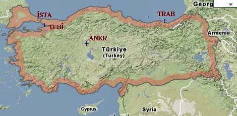
Figure 1: GNSS station Used in time series analysis

Hardware effect: Antennas meet signal moving in the atmosphere. To increase the accuracy of the height component, the calibration of the antennas is of great importance. The changing between the electrical center of the antenna and geometrical center antenna is not fi xed and the constant changing can be reduced or increased (Wübbena et al, 2006). Antenna radomes are used to protect signal quality due to external factors affecting the height component of the solution. This problem is currently under investigation (Hugentobler et al, 2006), (Schmid, 2006).

In the case of several weeks of discontinuation of the data in a station, extraction station periodic movement is not possible. For this purpose, different locations on the same station would be obtained if a different provision of GPS equipment and data can ensure the continuity of time series.

The other factors affecting the time series are as outlined below:

• The local meteorological effect, snow effect on the radome, local refraction, etc.,

• The seasonal effect, ocean stream (golfstream, labrador), tidal effect, glacial effect

• Earthquake effect (post-seismic, co-seismic and inter-seismic effect), fault movements

• Global plate movements, etc.

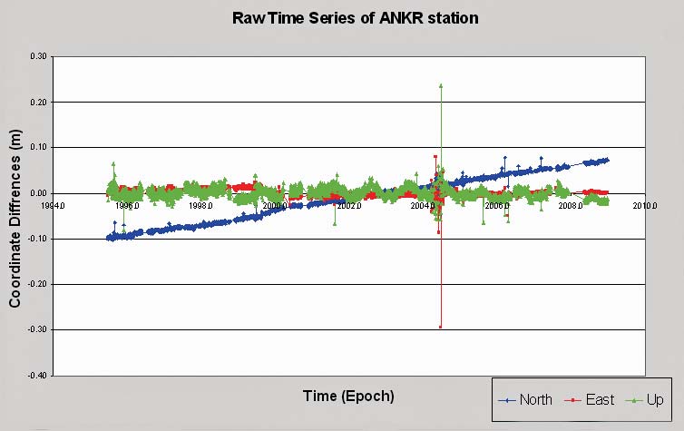
Figure 2: Time dependent changes in time series of ANKR station

Numerical application

Time series raw data of ANKR (20805M002), TUBI (20806M001), ISTA (20807M001) and TRAB (20808M001) stations have been used in the application (Figure 1). The raw data of N (North), E (East) and U (Up) local coordinates components of these stations have been provided from the Scripps Orbit and Permanent Array Center (SOPAC) GPS archive (web-1, 2009).

These local coordinates transform different Cartesian coordinates between reference epoch and measurement time epoch. These coordinates are composed of ITRF2005 reference epoch coordinates (X0 , Y0 , Z0 ) and daily local coordinates N, E, and U. Dates of the data cover the period from 26/06/1995 to 12/21/2008 in ANKR station, the period from 21/12/1995 to 08/05/1998 in TUBI station, the period from 26/12/1999 to 12/21/2008 in ISTA station, the period from 26/12/1999 to 28/11/2007 in TRAB station. For the N, E, and U coordinate components of the four stations, time series graphic has been drawn by Microsoft Excel on one graphic (Figure 2).

The Up component of four stations’ coordinate time series is similar to the periodic due to seasonal effects and it appears to have been seen to act. In addition, the unusual changes were noticed in Up component and it is assumed that these changes were caused by earthquakes. Firstly, the data interruptions of stations and gaps in time series were examined. For these gaps and interruptions, the time series were analyzed. The longterm discontinuities in the stations were analyzed separately for different ranges of epochs. Then the V-test was performed to determine outliers. Thus, the outliers were eliminated from time series. Then, in the height component of time series, periodic changes or seasonal effects were detected. So covering the years from 1995 to 2008 daily, the average temperature and pressure values of four stations were obtained from General Directorate of State Meteorology Affairs. Regression analysis of height component was performed according to the average pressure and average temperatures.

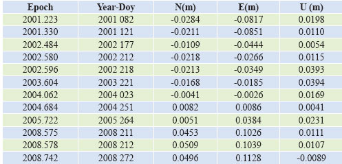
Table 1: Outliers of ISTA station time series

V – Statistics

In the measures made for sample the elements x1, x2, …., xn, V-statistics is used to examine the values, showing the greatest difference in whether belonging to the same set or not. (Yerci, 2002)

For the implementation of this test

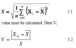
The size of the test is calculated by equation 8.2. Hypothesis is established. If the hypothesis is smaller than V table values, the hypothesis will be considered valid according to the V table with n measurements and α significance level.

N, E and U components of stations’ coordinates divided periods of 6 months. V – Statistics were performed separately for every period of application because of big range of data. The purpose of this test, one can understand whether the series are stationary or not when one investigates the long periodic time series. As a result values not outlying must stay in their time series. According to V-statistics, outliers were extracted from time series of four stations. In table 1,outliers of ISTA station are seen. There is much outlier in the other stations. But in this paper, other outlier tables are not presented due to the large quantity of data.

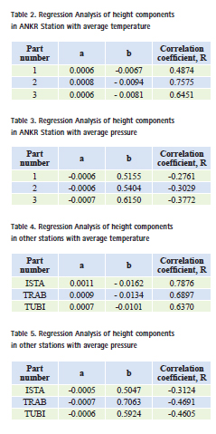
Regression analysis of height components in ANKR, TUBI, ISTA ant TRAB GNSS Stations with average temperature and pressure

Each station’s average temperature and pressure values with height components are shown in the graphics. e.g., in Figure 3 and Figure 4 TRAB station height components with temperature the y column has no unit, just two variables multiplied by specifi c coeffi cients for better understanding of the visual. Then, regression analysis of the height component was performed with accordance to the average pressure and average temperatures.

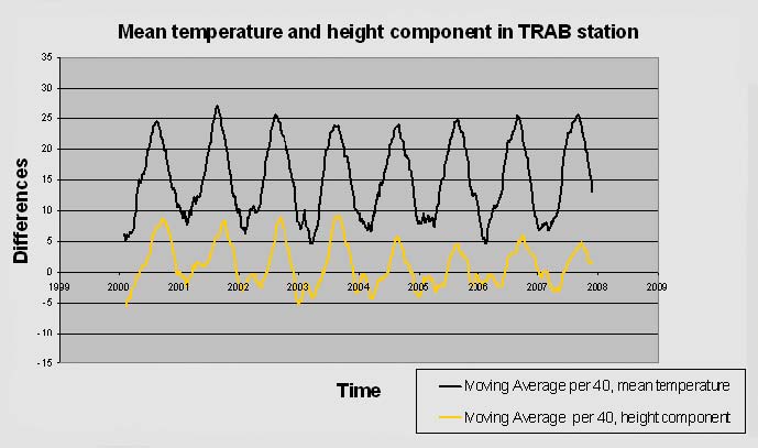
Figure 3: TRAB station’s height component and temperature

Regression is setting up of equality with the help of the known is thought to predict the form for later cases. In other words, regression was used to measure the relationship between two or more variables. Regression provides both descriptive and inferential statistics. If X is the only variable point to an incident, and dependent variable Y, between these two variables Y = f (X), the equation can be considered a link. It is assumed that, according to the result of a series of measurement, (X1, Y1), (X2, Y2), …, (Xn, Yn), values on a plane are obtained from specified points in quantitative cases. If the frequency distribution of these points is examined, the maximum frequencies of the classes are different straight line from X and Y axes and the values are dispersed around the straight line.

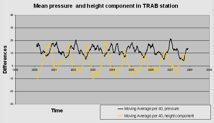
Figure 4. TRAB station’s height component and pressure

The distribution of these series may be non linear distribution. If one has the impression that a suitable non-linear distribution, it is named suitable curve. But if the distribution is linear, it is named as the linear regression line or adjusting line.

Regression analysis in ANKR station

ANKARA station data was divided into three parts because of long term gaps and regression analysis was made separately for the three sections. The fi rst part of ANKR station, the dates cover the period from 13.08.1999 to 26.06.1995. The second part, the dates cover the period from 17.03.2004 to 25.11.2000. The third part, dates cover the period from 30.11.2007 to 20.07.2004. In table 2, regression analysis coeffi cients and correlation coeffi cient with temperature are seen as y=ax+b regression equation. In table 3, regression analysis coefficients and correlation coefficient with pressure are seen as y=ax+b

Regression analysis in other stations

In table 4, in TUBI, ISTA, TRAB station, regression analysis coeffi cients and correlation coefficient with temperature are seen as y=ax+b regression equation. In table 3, regression analysis coefficients and correlation coeffi cient with pressure are seen as y=ax+b

Conclusions

One of the non secular behaviors often observed in GPS time series is the periodic variations with an annual period. The most obvious environmental factors with such period are temperature and pressure. Non-uniform temperature distributions and pressure of Earth surface due to solar radiation and tropospheric layer can cause thermal stress, expansion, subsidence and hence change in displacements and instability at the geodetic sites. In this study, we analyzed time series of GPS stations with temperature and pressure variations in a longer period of time. The GPS time series of stations lead us to assume that the displacement change of the GNSS station was due to temperature and pressure. Also there is a linear correlation between height component of station coordinates and temperature. On the other hand inverse correlation between height component of station coordinates and pressure has been seen.

References

Akalın, S., 1990, Business Statistics, Bayraklı Press, İzmir (in Turkish)

Akdeniz, H., A., 1998, Applied Statistics II, Nine September University, Faculty of Economics and Administrative Sciences, İzmir (in Turkish)

Allen, R.G.D., 1964, Statics for Economists, MC – Millan, UK

Dai, W.J., Ding, X.L., Li, Z.W., Kwok, K.C.S., Campbell, S., 2006, Tropospheric Effects on GPS Measurements, Hong Kong

Hugentobler U, van der Marel H, Springer T (2006) Identifi cation and Mitigation of GNSS Errors, IGS Workshop, Darmstadt.

Mann, S. P., 1995, Statistics For Business and Economics, Wiley, USA

Sincich, T., 1996, Business Statistics By Example, Prentice- Hall International Editions, fifth edition, USA

Pibon, M., 2002, Analysis of Periodic Behavior of GPS time Series at Pacoma Dam, California, Massachusetts Institute of Technology, Master of Science thesis,

Schmid R vd ,2006, Generation of igs05. atx –status quo, IGS Wokrshop, Darmstadt

Urschl C, Gurtner W, Hugentobler U, Schaer S and Beutler G (2005) Validation of GNSS orbits using SLR observations, Advances in Space Research, 2005, 412-417.

Wübbena G, Schmitz M, Boettcher G ,2006, Absolute GNSS antenna calibration with a robot: repeatabiltiy of phase variations, calibration of GLONASS and determination of carrier-tonoise pattern, IGS Workshop, Darmstadt.

Web-1, 2009, ftp://garner.ucsd. edu/pub/timeseries/