
| GNSS | |
Empirical orthogonal function based modelling of ionosphere using Turkish GNSS network
The study investigates ionospheric TEC variation over the Turkish region using 5 GNSS stations. The results showed that the overall TEC values display the trend of normal diurnal and annual TEC variations. |
|
|
|
|
Abstract
The study investigates ionospheric total electron content (TEC) variation over Turkey from the five selected global navigation satellite system (GNSS) stations situated in diverse parts of Turkey. The geomagnetic indices are used and observed TEC are modeled with the technique known as Empirical orthogonal function (EOF). It is valuable to note that the correlation coefficient between observed GNSS TEC values and EOF TEC values varies from 0.8020 to 0.9394. The root means square error (RMSE) values between observed GNSS TEC values and EOF TEC lie between 3.1665 TECU to 4.4220 TECU. These results show that the EOF model performs quite well in the Turkish region and can present the model TEC variations perfectly. Finally, these GNSS observed and EOF- predicted TEC values along with geomagnetic indices are studied with the tropospheric wind speed. The results showed that both observed and modeled TEC have very low correlations with tropospheric wind speed and do not provide any significant value. Hence, we concluded that the ionospheric region is not affected by tropospheric wind speed. It happens because the tropospheric wind speed is a matter of the lower troposphere and its atmospheric pressure while the ionosphere is far from the earth and depends upon the number of free electrons.
1. Introduction
The ionospheric region that affects the global navigation satellite system (GNSS) signals is a major error source for single point positioning measurements. The ionospheric range error, which is directly related to the ionospheric total electron content (TEC) keeps on changing and depends upon the solar and geomagnetic activities, geographical or geomagnetic coordinate systems, local and universal time, and seasonal effects (Júnior et al., 2020; Ansari et al., 2018; Seok et al., 2022; Sharma et al., 2020). The ionospheric delay gradient magnitude occurs often and directly influences the values of TEC; so that an error in positioning could be reachable up to several 10 m (Seeber, 2003). Hence modeling and prediction of spatiotemporal ionospheric TEC error is very necessary for the applications of weather investigations. Since the ionosphere contains a dispersive medium, hence first-order approximation delay in the ionosphere can be estimated by applying simultaneous measurements at two different frequencies. However, this approach is not successful for the single frequency operations (Júnior et al., 2020. Their many techniques and forecasting models have been developed such as quasi-experimental model (IRI, IRI Plus, NeQuick2) and theoretical hypothetical models such as Auto-regressive Moving Average, Empirical Orthogonal Function and others (Bilitza et al., 2017; Jakowski et al., 2011; Nigussie et al., 2012; Tuna et al., 2014; Zhang and Moore, 2015; Ansari et al., 2019). These models are used in remote areas where no device is available. In general, it is expected from empirical models that they will reflect the actual ionospheric features, however, they come across numerous kinds of modeling limitations depending upon the data used to reconstruct them such as considered instantaneous space weather situations, implicated techniques, etc. In contrast to the direct reconstruction, modes of principal component analysis related to the physics of the ionosphere can be utilized for various conditions. They can duplicate the desired result and present empirical results at some level. Hence, these kinds of models are still needed to describe the variability of the ionosphere.
The Empirical Orthogonal Function (EOF) method, which is based on principal component analysis, reported improved ionospheric prediction results. Ercha et al. (2012) established a global ionospheric TEC model based on EOF analysis using global ionospheric maps (GIM) data from one decade (1999–2009). According to them, overall TEC variation including the influence of geomagnetic activity and solar radiation toward TEC can be presented very well by the characteristics of EOF associated coefficients and base functions. Therefore, a global TEC model was established incorporating the EOF of the TEC time series. The modeled TEC time series was validated with the observed TEC to check the accuracy and quality of the model, which pointed out that the model can reflect the spatiotemporal feature of the global TEC variation. Later several studies that followed this EOF model validated the outcome at the local level (Ansari et al., 2019; Jamjareegulgarn et al., 2020; Dabbakuti et al., 2016). Ansari et al. (2019) used ionospheric data from South Korea and presented an EOF-modeled study of the ionosphere. They used 14 GNSS stations covering the area of South Korea from 2010 to 2017. They included the PCN index including the other geomagnetic indices such as Ap, Dst, and F10.7, and evaluated their EOF-based modeled TEC values with NeQuick-2 and IRI-2016 models. They noticed that their results showed better performance compared to the IRI and al. (2020) presented their EOF method modeled ionospheric study over the region of Nepal using three years (2017–2019) TEC observations from 5 GNSS stations. Both modeled and observed TEC values with the global ionospheric maps (GIM) models are compared. They found that the correlation coefficient of observed GNSS TEC with EOF-modeled TEC was higher compared to the correlation coefficient of observed TEC with GIM TEC values. Dabbakuti et al. (2016) constructed an EOF model using data from IISC (India) IGS station during the extended period of 2009–2016 in the 24th solar cycle. The modeled TEC was validated during day and night-time as well as under distinct geomagnetic and solar activity situations. The reliability and validity of the EOF model were verified with the comparison of standard global IRI 2016 and SPIM models. They noticed that the EOF model performance was relatively better during the period of high solar activity compared to the period of low solar activity.
Although the studies based on the above discussion enhance the utility of ionospheric variations. However, to understand the relative contribution of neutral winds, neutral temperature, neural electric field, and neural density periodicities on the ionosphere, further developments, more simulated models, and additional data are required. The ionospheric region which lies between 50 and 1000 km above the earth’s surface includes the mesosphere (50–85 km), the thermosphere (100–690 km), and the partial part of the Exosphere (690–10,000 km). Since during the estimation of TEC, it is assumed that the ionosphere to be a thin shell and located at 350 km altitude above the Earth, hence in the current study, we investigated the geomagnetic activity and its relationship with tropospheric wind speed in the mesospheric and thermosspheric regions of Turkey. The new findings of the study introduce a solar-terrestrial relation that yields in the ionosphere. We used GNSS data from five GNSS stations across Turkey covering the one year of January 2015 to December 2015. First, the relation between GNSS TEC including geomagnetic indices with tropospheric wind speed was presented. A small description of data collection and utilized geomagnetic indices has been given in Section 2. In the next step observed TEC was modeled by using the EOF method and their comparison result is presented. A summary of the proposed EOF method can be seen in Section 3. Later this EOF modeled TEC again compared with the tropospheric wind speed and the obtained results are explained. The result and discussion of the whole study have been presented in Section 3. The conclusion and future of the study have been written in Section 4.
2. Data collection and method of processing
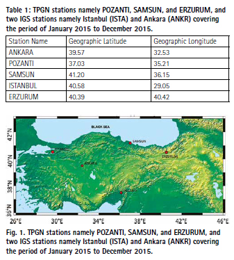
The paper presents ionospheric TEC variation using the GNSS data from the Turkish Permanent GNSS Network (TPGN) including the Turkish IGS stations. TPGN is a huge GNSS network of Turkey containing around 150 stations across all over Turkey. This study includes three TPGN stations namely POZANTI, SAMSUN, and ERZURUM, and two IGS stations namely Ankara (ANKR) and Istanbul (ISTA) from January 2015 to December 2015 (Fig. 1, Table 1). The TPGN data has been accessed from the TUSAGA-Aktif website (https://www.tkgm.gov. tr/tr/ icerik/tusaga-aktif-0) and while IGS data was downloaded from the CDDIS website (ftp://cddis.gsfc.nasa.gov/).
To retrieve the TEC data from the RINEX f iles, three major steps are required. First, is the preprocessing of RINEX observations to compute the TEC values, the second task is the computation of TEC and the third is the data presentation to be used for research. IONOLAB TEC (www.io nolab.org) software successfully provides all these steps in online mode. The Reg-Est, which applies IONOLAB-BIAS and is programmed by JAVA language, began to use an online trial version of TEC estimation in 2007. The Scientific and Technological Research Council of Turkey (TUBITAK) granted this program and IONOLAB-BIAS has been developed further for near real-time space weather applications known as IONOLAB-TEC. The IONOLAB-TEC method is a regularized TEC (D-TEI) algorithm and was developed to estimate TEC by utilizing all GNSS signals measured at a period on the selected day. In the current study, we have used IONOLAB- TEC software to retrieve the TEC and tried to detect abnormal ionospheric activities over Turkey using the GNSS data from Turkey stations.
In the current study, we also used the solar and geomagnetic indices data such as the Dst Index, F10.7, Ap Index, IMF-B, Kp Index, and sunspot number (R) including the tropospheric wind speed accessed from the server of NASA (omniweb. gsfc.nasa.gov). Including. These indices are used to measure the geomagnetic activity, for the signature of the ionospheric response and magnetosphere of the Earth to solar forcing. They played a considerable role in describing the magnetic formation of the ionized Earth environment. Detailed information about geomagnetic indices can be studied by Menvielle et al. (2010).
3. Summary of EOF modeling
Let us suppose the matrix of observed TEC measurement is given by X, arranged in the order such that its diurnal variation presents a row of the matrix while hourly variation shows a column of the matrix X. In the current study, only one year (2015) of data has been used, hence there will be 365 rows and 24 columns in the given observed matrix of X. This matrix is not square; hence we can obtain a square matrix of Z like this:
![]()
If we decompose the Z matrix in terms of the base function (Ek ) and the associated coefficient (Ak ). The original data set of X can be written in following form:
4. Result and discussion
4.1. Ionospheric TEC and geomagnetic indices
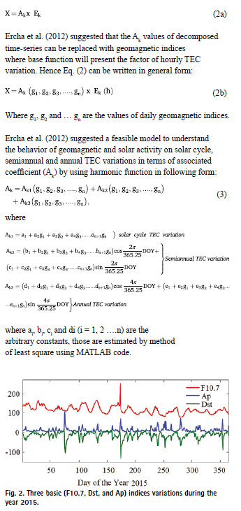
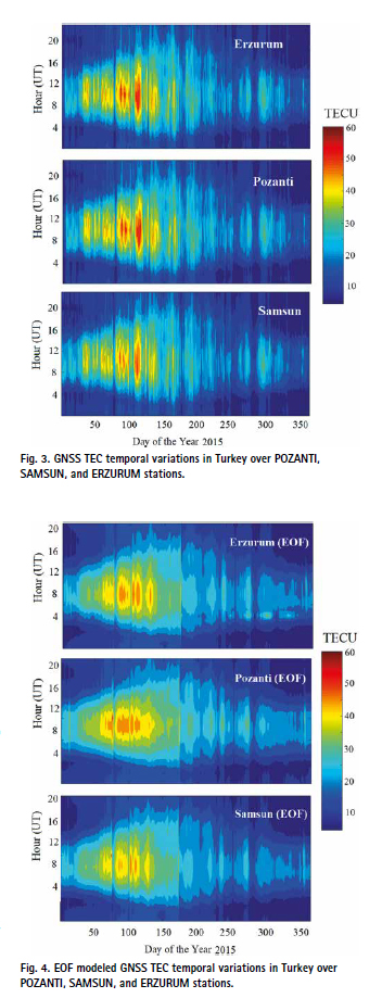
The geomagnetic field is responsible for the regulation of ionospheric variation, which is the fundamental parameter of the ionosphere (Council, 1993). The basic indices used to express the changes in the geomagnetic field are the indices F10.7, Dst, Ap, Kp, and AE indices (Atıcı et al., 2020). We plotted three basic (F10.7, Dst, and Ap) indices variations during the year 2015 as shown in Fig. 2. The appearance of one peak (lower side for Dst, upside for F10.7 and Ap and) can be seen during the period of selection. These peaks point out the time of high solar activity (HSA) on 173 days of the year 2015 when the Dst value reached – 133 nT and F10.7 became 255 s.f.u. GNSS observed ionospheric variation is investigated to understand its attributes over Turkey. Temporal variations in GNSS VTEC over POZANTI, SAMSUN, and ERZURUM have been shown in Fig. 3. On the day of HSA, the VTEC showed 40.15 TECU at POZANTI, 36.32 TECU at SAMSUN and 38.53 TECU at ERZURUM. Regarding the X-axis of the plot, the diurnal pattern of VTEC variation shows some low VTEC values (about 25 TECU) during the start of the year, which start to increase more during the days of 50–60 and reach up to 40 TECU at almost all stations. This variation showed a few low values during the day of 200 and later decreased more and became the lowest (about 18 TECU) at the end of the year. Regarding the Y-axis which are hourly plots, the VTEC showed the lowest values around 15 TECU at the statement of the day at 04:00 UT and started to increase till 08:00 UT, reaching up to 25 TECU. The plots showed the highest value between 06:00 UT to 14:00 UT which is highest at noon UT. This is notable because this highest value at noon UT keeps on varying for up to a whole year. Overall TEC values display the trend of normal diurnal and annual TEC variations. This happens due to the revolution and rotational motion of the Earth around the Sun (Rat-nam et al., 2017).
4.2. EOF modeled TEC variation
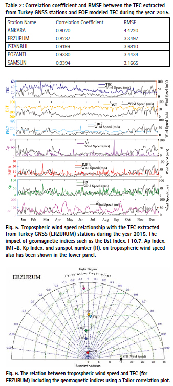
This is clear from Eq. (3), if we take one geomagnetic index analysis, we need to handle 10 constant coefficients, and if we take two geomagnetic indices, there will be 15 constants, that need to be handled. To avoid a more complex analysis, we selected three basic indices (F10.7, Dst, and Ap) and estimated 20 constant coefficients by using the least square method. There are several studies already done, that used these three indices only in their EOF analysis (Dabbakuti et al., 2016; Jamjareegulgarn et al., 2020). In the current analysis, we used these three basic indices (F10.7, Dst, and Ap) as described in Fig. 2 and predicted EOF TEC values at stations i.e., Ankara, Erzurum, Istanbul, and Pozanti (Fig. 4). Here it is difficult to compare Fig. 4 with the corresponding GPS TEC of Fig. 3 in the first view, as they do not exhibit the same kind of variation. Hence, the EOF TEC values are used to do a comparative analysis with the observed GNSS TEC values by using the correlation coefficient and RMSE as shown in Table 2. It is valuable to note that the correlation coefficient of observed GNSS TEC values with EOF TEC values are 0.8020 at Ankara, 0.8287 at Erzurum, 0.9199 at Istanbul, 0.9380 at Pozanti, and similarly 0.9394 at Samsun sites (Table 2). The result shows that the correlation coefficients have different values at each station. This type of variation is nothing but because of some data issues. Some station data variations were affected badly due to any physical cause, hence the performance of the EOF method could not become proper. In the next step, we estimated RMSE between observed TEC and EOF TEC values as shown in Table 2. This is clear from the Table that the RMSE varies from 3.1665 TECU (Samsun) to 4.4220 TECU. These values are very low with a small variation at each station. The station which has a high correlation shows low RMSE and the station which has a low correlation shows high RMSE. In conclusion, it can be said that the EOF model performs quite well and can present the model TEC variations perfectly.
The accuracy of the EOF model has been already tested in various regions. For example, Jamjareegulgarn et al. (2020) noticed that the correlation coefficients between observed TEC and EOF TEC over the Nepal region (2017–2019) was up to 0.978, indicating the perfectness of the model. Ansari et al. (2019) used data from January 2010 to December 2017 and computed the correlation and best-fit line of GNSS-VTEC with EOF TEC. The EOF-VTEC was highly correlated (~0.97) at all stations, reflecting the realistic modeling and dependency of geographical as well as geomagnetic variation characteristics of TEC. Dabbakuti and Ratnam (2016) investigated ionospheric variability in a low-latitude region of India based on the EOF. The accuracy of the EOF model was validated by the evaluation of observational TEC data with International Reference Ionosphere (IRI) 2012 models. The EOF model coefficients for each GNSS station showed a strong correlation with the IRI models and also described the correlation between the impacts of the level of geomagnetic activity on the ionosphere. The correlation coefficients for the first three EOFs were more than 0.95. Li et al. (2019) used the EOF decomposition technique and studied the spatiotemporal characteristics of TEC from 2007 to 2016 in China. The results showed that the first-order EOF component dominated the overall TEC variation because it accounted for 97.35% of the total variance. However, in the current study, the correlation coefficient of observed GNSS TEC values with EOF TEC values is low (0.80 0.9199) compared to the above studies. These low correlation coefficients are happening because of badly affected data due to any physical causes. This type of decreasing performance of the EOF method points out some limitations of the EOF model. Finally based on the above discussion we can conclude that the EOF-based TEC model can demonstrate the temporal and spatial variation characteristics of TEC, and the EOF based model can obtain significantly smaller modeling errors and achieve better performance in terms of TEC modeling.
4.3. Tropospheric wind speed and geomagnetic indices
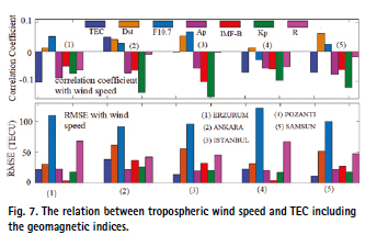
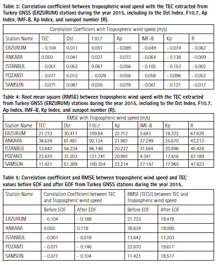
The solar radiation warms the air in the surrounding region, and then this warm air rises and creates a low pressure in the region. In the case of large-scale circulation, the tropospheric wind speed simply depends upon the difference in temperature and pressure (Ansari, 2016; Ansari et al., 2021). To understand the effect of tropospheric wind speed on the available electron densities of the ionospheric region, we studied the tropospheric wind speed relationship with the TEC extracted from Turkey GNSS (ERZURUM) stations during the year 2015 (Fig. 5). The impact of geomagnetic indices such as the Dst Index, F10.7, Ap Index, IMF-B, Kp Index, and sunspot number (R), on tropospheric wind speed also has been shown in Fig. 5. Here we are showing only one plot (ERZURUM only) to save the space because all other plots will be almost the same. Since the tropospheric wind speed is a vector quantity, hence the tropospheric wind speed average and its direction always depict a wider difference compared to the instantaneous value of speed and direction (Lolis et al., 2018; Ansari et al., 2021). To avoid such a type of wider difference analysis we choose the timing of TEC and tropospheric wind speed at noon only. The timing of noon is chosen because generally, TEC provides the highest variation at this due to the solar radiation. It is clear from Fig. 5, that the tropospheric wind speed varies from 0 to 70 m/s which has no common trend with TEC (first panel). Similarly, other geomagnetic panels such as the Dst Index, F10.7, Ap Index, IMF-B, Kp Index, and R also do not provide any kind of trend with tropospheric wind speed. The relation between tropospheric wind speed and TEC including the geomagnetic indices has been studied using a Tailor correlation plot as shown in Fig. 6 (for ERZURUM only) and Fig. 7 (for other stations). These relationships in terms of correlation coefficient have been tabulated in Table 3. All the correlation coefficient values from the table clearly showed less than or equivalent to 0.10 which means they have no relationship or very negligible effect of tropospheric wind speed on TEC or geomagnetic values. The tropospheric wind speed is a matter of lower troposphere and its atmospheric pressure while the ionosphere is very far from the earth and depends upon the number of free electrons, hence without a doubt they are not affecting the ionospheric region. For more confirmation, we studied root mean square error (RMSE) with tropospheric wind speed and geomagnetic parameters as shown in Table 4. This is notable that RMSE for each parameter is very high which again indicates a negligible relation of tropospheric wind speed with the ionosphere.
4.4. EOF modeled TEC and tropospheric wind speed
We used the EOF method and predicted TEC at all selected Turkey stations by using observed TEC and three basic geomagnetic indices (F10.7, Dst, and Ap). It means EOF TEC is a function of TEC, F10.7, Dst, and Ap. To analyze the relation between modeled TEC and tropospheric wind speed, the correlation coefficient, and RMSE at noon of each station have been estimated as shown in Table 5. It is clear from the Table that the correlation after applying EOF is less than or equivalent to 0.10 which means they have no relationship or very negligible effect of tropospheric wind speed on EOF TEC. The RMSE for EOF is also very high which again indicates negligible relation of EOF TEC with tropospheric wind speed. There is a little bit of change before EOF (observed TEC) and after the implication of EOF, but not obtained results do provide any significant information. Since tropospheric wind speed does not have any kind of relationship with observed TEC and other geomagnetic indices, hence the same kind of negligible relationship was expected with EOF TEC, because EOF TEC is a function of TEC and geomagnetic indices.
5. Conclusions
The study investigates ionospheric TEC variation over the Turkish region using 5 GNSS stations. The results showed that the overall TEC values display the trend of normal diurnal and annual TEC variations. This happens due to the revolution and rotational motion of the Earth around the Sun. The EOF TEC values are used to do a comparative analysis with the observed GNSS TEC values and found that the correlation coefficient of observed GNSS TEC values with EOF TEC values are 0.8020 at Ankara, 0.8287 at Erzurum, 0.9199 at Istanbul, 0.9380 at Pozanti, and similarly 0.9394 at Samsun sites. These variations of correlation coefficients are nothing but because of some data issues. The tropospheric wind speed at the selected location of GNSS sites is correlated before EOF and after EOF model TEC. All the correlation coefficient values from the table clearly showed less than or equivalent to 0.10 which means they have no relationship or very negligible effect of tropospheric wind speed on TEC or geomagnetic values. Similarly, other geomagnetic panels such as the Dst Index, F10.7, Ap Index, IMF-B, Kp Index, and R also do not provide any kind of trend with tropospheric wind speed. This indicates that the tropospheric wind speed is not related to the ionospheric conditions because the tropospheric wind speed is a matter of the lower troposphere and its atmospheric pressure while the ionosphere is far from the earth and depends upon the number of free electrons.
Funding
The research was funded by the Warsaw University of Technology within the Excellence Initiative: Research University (IDUB). contribution statement Kutubuddin Ansari: Writing – review & editing, Writing – original draft, Data curation, Conceptualization. Janusz Walo: Writing – review & editing. Selcuk Sagir: Writing – review & editing. Kinga Wezka: Writing – original draft. Declaration of competing interest The authors declare that they have no conflict of interest.
Data availability
Data will be made available on request.
References
Atıcı, R., Aytas¸, A., Sa˘gır, S., 2020. The effect of solar and geomagnetic parameters on total electron content over Ankara, Turkey. Adv. Space Res. 65, 2158–2166. https:// doi.org/10.1016/j.asr.2019.07.018.
Ansari, K., Panda, S.K., Corumluoglu, O., 2018. Mathematical modelling of ionospheric TEC from Turkish permanent GNSS Network (TPGN) observables during 2009–2017 and predictability of NeQuick and Kriging models. Astrophys. Space Sci. 363 (3), 1–13. https://doi. org/10.1007/s10509-018-3261-x.
Ansari, K., Park, K.D., Panda, S.K., 2019. Empirical orthogonal function analysis and modeling of ionospheric TEC over South Korean region. Acta Astronaut. 161, 313–324. https://doi. org/10.1016/j.actaastro.2019.05.044.
Ansari, K, 2016. Monitoring and prediction of precipitable water vapor using GPS data in Turkey. Journal of Applied Geodesy 10 (4), 233–245. https:// doi.org/10.1515/jag- 2016–0037.
Ansari, K., Bae, T.S., Lee, J., 2021. Spatiotemporal variability of total cloud cover measured by visual observation stations and their comparison with ERA5 reanalysis over South Korea. Int. J. Climatol. 41 (S1), E1757–E1774. https://doi.org/10.1002/ joc.6805.
Bilitza, D., Altadill, D., Truhlik, V., Shubin, V., Galkin, I., Reinisch, B., Huang, X., 2017. International Reference Ionosphere 2016: from ionospheric climate to real-time weather predictions. Space Weather 15, 418–429. https://doi.org/10.1002/ 2016SW001593.
Council, N.R., 1993. The National Geomagnetic Initiative. The National Academies Press, Washington, DC. https://doi.org/10.17226/2238.
Dabbakuti, J.K., Ratnam, D.V., 2016. Characterization of ionospheric variability in TEC using EOF and wavelets over low-latitude GNSS stations. Adv. Space Res. 57 (12), 2427–2443. https://doi. org/10.1016/j.asr.2016.03.029.
Ercha, A., Zhang, D., Ridley, A.J., Xiao, Z., Hao, Y., 2012. A global model: empirical orthogonal function analysis of total electron content 1999–2009 data. https:// doi. org/10.1029/2011JA017238.
Jakowski, N., Mayer, C., Hoque, M.M., Wilken, V., 2011. Total electron content models and their use in ionosphere monitoring. Radio Sci. 46 (6) https:// doi.org/10.1029/ 2010RS004620.
Jamjareegulgarn, P., Ansari, K., Ameer, A., 2020. Empirical orthogonal function modeling of total electron content over Nepal and comparison with global ionospheric models. Acta Astronaut. 177, 497–507. https://doi. org/10.1016/j. actaastro.2020.07.038.
Júnior, P.D.T.S., Aquino, M., Veettil, S.V., Alves, D.B.M., da Silva, C.M., 2020. Seasonal analysis of Klobuchar and NeQuick G single-frequency ionospheric models’ performance in 2018. Adv. Space Res. https://doi. org/10.1016/j.asr.2020.11.013.
Li, S., Zhou, H., Xu, J., Wang, Z., Li, L., Zheng, Y., 2019. Modeling and analysis of ionosphere TEC over China and adjacent areas based on EOF method. Adv. Space Res. 64 (2), 400–414. https://doi. org/10.1016/j.asr.2019.04.018.
Lolis, C.J., Kotsias, G., Bartzokas, A., 2018. Objective definition of climatologically homogeneous areas in the southern Balkans based on the ERA5 data set. Climate 6 (4), 96 doi:10.3390/cli6040096.
Menvielle, M., Iyemori, T., Marchaudon, A., Nos´e, M., 2010. Geomagnetic indices. In: Geomagnetic Observations and Models. Springer Netherlands, Dordrecht, pp. 183–228.
Nigussie, M., Radicella, S.M., Damtie, B., Nava, B., Yizengaw, E., Ciraolo, L., 2012. TEC ingestion into NeQuick 2 to model the East African equatorial ionosphere. Radio Sci. 47 https://doi. org/10.1029/2012RS004981.
Ratnam, D.V., Sivavaraprasad, G., Devi, N.L., 2017. Analysis of ionosphere variability over low-latitude GNSS stations during 24th solar maximum period. Adv. Space Res. 60 (2), 419–434. https://doi. org/10.1016/j.asr.2016.08.041.
Seok, HW, Ansari, K, Panachai, C, Jamjareegulgarn, P, 2022. Individual performance of multi-GNSS signals in the determination of STEC over Thailand with the applicability of Klobuchar model. Advances in Space Research 69 (3), 1301–1318. https://doi. org/10.1016/j.asr.2021.11.025.
Sharma, SK, Singh, AK, Panda, SK, Ansari, K, 2020. GPS derived ionospheric TEC variability with different solar indices over Saudi Arab region. Acta Astronautica 174, 320–333. https://doi.org/10.1016/j. actaastro.2020.05.024.
Seeber, G., 2003. Satellite Geodesy, 2nd Completely Revised and Extended Edition, vol. 10785. Walter de Gruyter GmbH & Co. KG, pp. 303–304.
Tuna, H., Arikan, O., Arikan, F., Gulyaeva, T.L., Sezen, U., 2014. Online user-friendly slant total electron content computation from IRI Plas: IRI-Plas-STEC. Space Weather 12, 64–75. https://doi.org /10.1002/2013SW000998.
Zhang, Z., Moore, J.C., 2015. Chapter 6 – empirical orthogonal functions. In: Zhang, Z., Moore, J.C. (Eds.), Mathematical and Physical Fundamentals of Climate Change. Elsevier, Boston, pp. 161–197. https:// doi.org/10.1016/B978-0 12-800066- 3.00006-1.
© 2024 The Author(s).
Orginally published in Journal of Atmospheric and Solar–Terrestrial Physics 261 (2024) 106294. Published by Elsevier Ltd.
This is an open access article under the CC BY license (http://creativecommons. org/licenses/by/4.0/).
The article is republished with the permission from the author.


 (3 votes, average: 2.33 out of 5)


Leave your response!