
| Surveying | |
Australia’s first state-wide airborne gravity model
This paper presents some background on airborne gravimetry, introduces the NSW Gravity Model and outlines the benefits it will provide to the surveying profession and wider community. |
 |
|
 |
|
 |
|
Gravity is not only a fundamental force in physics, surveying and geodesy but also crucial for life in general. It pins our atmosphere to the Earth, keeps our feet on the ground and causes fluids to f low downhill. Today’s modern Australian surveyor regularly works with two types of heights: ellipsoidal heights referred to the Geocentric Datum of Australia 2020 (GDA2020, see Harrison et al., 2024) and physical heights referred to the Australian Height Datum (AHD), Australia’s first and only legal vertical datum (Janssen and McElroy, 2021). A new third option, the Australian Vertical Working Surface (AVWS), offers an alternative for early adopters and/or precise users requiring higher-quality physical heights (current accuracy about 4-8 cm) than those AHD can provide (accuracy about 6-13 cm) (ICSM, 2021). Global Navigation Satellite System (GNSS) users can access AVWS by applying the Australian Gravimetric Quasigeoid (AGQG, see Featherstone et al., 2018) model to their GDA2020 ellipsoidal heights, just like AUSGeoid2020 is used to obtain AHD heights (Featherstone et al., 2019).
Both geoid models can be improved by collecting high-quality, consistent and evenly distributed gravity measurements to complement and update the existing geoscientific datasets, which are mostly based on regional-scale, historical precompetitive datasets and modern targeted data capture for mineral resource exploration (consisting of a combination of land-based and airborne gravity data collected over several decades). This improvement is best achieved via airborne gravity measurements. A big advantage of gravity data is that it (generally) does not change over time, so it can be captured once and used many times for many diverse applications, provided it is available at sufficient quality and density.
Of particular interest to surveyors in New South Wales (NSW) is that DCS Spatial Services, a unit of the NSW Department of Customer Service (DCS), hosts the largest state-owned and operated GNSS Continuously Operating Reference Station (CORS) network in Australia (Janssen et al., 2016). To unlock the full potential of CORSnet-NSW, a state-wide gravity model is required to improve both geoid models and deliver consistent, higher quality heighting across the state.
This paper introduces the NSW Gravity Model, the nation’s first state-wide gravity model produced from a survey captured in a single airborne campaign, which was delivered by DCS Spatial Services in collaboration with the Geological Survey of NSW and Geoscience Australia (Janssen et al., 2025). It presents some background on airborne gravimetry, discusses data collection and processing, and outlines the benefits this model will provide to the surveying profession and wider community, with gravity data made freely available to the public for the benefit of all.
Airborne gravimetry
Gravity is the force acting on a body on or near the Earth’s surface, which is a combination of the gravitational force (the force of attraction between two masses) and the centrifugal force (the apparent force caused by the uniform circular motion of a body about a fixed point) of the Earth’s rotation. In the absence of friction and other forces,it is the rate at which objects will accelerate towards each other. At the Earth’s surface, gravity (acceleration) is approximately 9.8 m/s2, with absolute gravitational acceleration varying across Australia between 9.780 m/s2 in northern Australia and 9.805 m/s2 in southernmost Tasmania (Kennett et al., 2018).
In principle, gravity can be measured using an accelerometer, which houses a proof mass that is restricted to movement along a sensitive axis and a restraining device (e.g. a spring). The mass is supported by the restraining device and displaces with respect to an equilibrium position when subject to acceleration. Knowing the relationship between the displacement and the restoring force applied to the mass (e.g. due to Hooke’s law), the accelerometer provides a measure of the force required to counter the force due to accelerations acting on the mass. Gravity is generally measured in units of gal (1 Gal = 1 cm/s2) or milligal (mGal).
An absolute gravity meter (or gravimeter) measures gravity at a single location, which is currently restricted to ground based acquisition. It determines the actual value of the gravitational acceleration, generally by measuring the speed of a falling mass in vacuum using a laser beam and optical interferometry. A relative gravimeter is much more common and measures the difference in gravity between two locations via ground-based, shipborne, airborne or satellite-based acquisition, generally using a spring supporting a proof mass. To be truly effective, this must include acquisition at one or more sites where absolute gravity is known (e.g. an existing gravity mark at the airport where the aircraft is based). Today’s airborne gravimetry systems can be separated into traditional airborne gravity systems and gradiometer systems. Both are very complex, requiring a multitude of sophisticated corrections and filtering to extract the desired gravity signal from the measured values.
Airborne gravity systems measure the sum of the aircraft accelerations and the Earth’s gravitational field. In simple terms, subtracting the GNSS derived vertical accelerations of the aircraft from the total vertical gravity measured by the instrument will provide residual gravity. In practice, additional corrections are required to account for platform misalignment (tilt), lever arm (spatial relationship between the GNSS antenna, airborne gravimeter and any other equipment used within the aircraft), horizontal accelerations, drift, Eötvös effect (relative change of the centrifugal force of the Earth’s rotation due to being on a moving platform) and minor temperature and pressure variations (Wooldridge, 2010).
The reduction of airborne gravity data requires the use of low-pass filters because the long- to medium-wavelength signal is of interest, while most noise has a short wavelength (i.e. high frequency) and corresponds to limitations in removing inertial accelerations of the aircraft using band-limited GNSS data. Factors influencing resolution and accuracy include aircraft speed, altitude and the spacing of flight lines. While precision from airborne data can be assessed well (using repeat tracks, adjacent tracks, tie lines or crossovers, and grid comparisons), accuracy is much harder to determine (using models, satellite data or ground data) because the true value is not really known, although good global models exist (Preaux, 2016)
Airborne gravity gradiometer systems measure the gradient of the Earth’s gravitational field independent of aircraft accelerations. They utilise spinning discs equipped with multiple accelerometers, which measure two or more components of the gravity gradient tensor depending on the number of discs and their orientation. The discs rotate which makes the gravity signal periodic of short temporal baselines, so that the gravity signal can be separated from drift in the accelerometers. The gradients measured at different locations are then transformed to vertical gravity. Gravity gradients are measured in units of Eötvös (Eö), where 1 Eö = 10-9/s2= 0.1 mGal/km, i.e. a variation of 1 mGal/ km is 10 Eö (Fairhead et al., 2017).
Airborne gravity gradiometer systems are generally more accurate (higher resolution) and more robust because they are less sensitive to aircraft accelerations, but also much more expensive. They must detect very small differential gravitation signals over a short baseline. This requires accounting for scale factor errors and accelerometer bias drift (accelerometers are not perfectly matched), alignment errors (sensitive axes of the accelerometers are not parallel), asymmetry of the configuration (measurement point is not the centre of mass of the accelerometer pair) and self-gradients (the gradient f ield is changed due to the rotation of the aircraft about the stabilised platform hosting the instrument), which is mostly achieved through calibration and filtering (Jekeli, 2003).
Data collection & processing
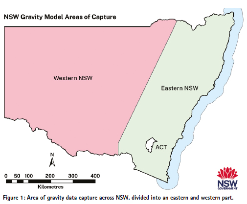
NSW is a large state (about 1.5 times the size of France) encompassing an area of 800,000 km2 and a coastline of 2,100 km in length, with terrain varying from vast plains to rugged mountainous areas (elevations up to 2,228 m at Mt Kosciuszko). In order to facilitate efficient data collection utilising two expert contractors, the area of interest (which also includes the offshore area up to 50 km from the east coast) was divided into two parts: Eastern NSW and Western NSW (Figure 1). These two parts (each completed by a single contractor) were then stitched together to produce the final products. The total area of capture amounted to 820,000 km2, also covering another jurisdiction, the Australian Capital Territory (ACT), in its entirety.
Eastern NSW
Sander Geophysics was contracted to complete Eastern NSW (Sander Geophysics, 2024). This area covers slightly more than the eastern third of NSW, including the Great Dividing Range, the ACT and the offshore margin up to 50 km from the coast (which includes the continental shelf). In the west, it is bordered roughly by a line through the towns of Narrabri, Dubbo and Wagga Wagga.
The principal survey traverse lines were oriented at 20º clockwise from north and spaced at 2,250 m onshore and 2,500 m offshore. A selected area of denser infill lines (mainly covering the north-east of NSW) resulted in lines spaced 1,125 m onshore and 1,250 m offshore. Tie lines for crossover checking used to level the survey data were oriented east-west at 90º and spaced at 75 km. A drape surface used to guide the aircraft’s height above the ground was created, considering the terrain and the performance of the aircraft at the expected altitudes and estimated temperatures. The survey was flown with a target clearance of 160 m above ground level, following the drape. Due to air traffic control restrictions, the area around Sydney Airport was flown at higher altitudes (between 518 m and 610 m). The target average ground speed was 60 m/s.
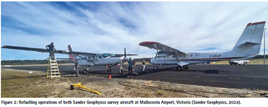
Due to safety and environmental considerations, the survey was split into ‘hostile’ and ‘non-hostile’ areas. The western, non-hostile area was flown with a single-engine Cessna C208B Grand Caravan, while the eastern ‘hostile’ area (i.e. densely populated and offshore areas) was flown using a twin-engine de Havilland DHC-6 Twin Otter (Figure 2). Bases of operation were Orange, Cessnock, Tamworth and Kempsey, as well as Mallacoota, Victoria.
Production flights commenced in August 2022 and lasted for 16 months, with data acquisition spanning all four seasons. Summer weather was usually hot and dry but occasionally interrupted by wet spells with significant rainfall. In autumn, winter and spring, higher elevations experienced long periods of wet weather with low visibility, causing many days when survey flights were not possible. On a few occasions, large parts of the survey area were subject to heavy rains and flooding. A total of 242 flights were carried out to complete the planned 223,318 line kilometres.
The position of the temporary GNSS reference stations at each airport was calculated via Precise Point Positioning (PPP) corrections using the algorithm developed by Natural Resources Canada for its CSRS-PPP online positioning service (NRCan, 2025), which has been incorporated into the suite of software used.
Gravity data was collected with the Airborne Inertially Referenced Gravimeter (AIRGrav) system, which was designed by Sander Geophysics specifically for the unique characteristics of the airborne environment. The relative airborne data was tied to absolute gravity by connecting to a nearby Australian Fundamental Gravity Network (AFGN) station, typically already established at the airport. The gravimeter was then calibrated at the aircraft’s exact parking location daily to the local gravity value.
Repeat test lines, planned and established in consultation with DCS Spatial Services, were flown periodically during the data acquisition to demonstrate the accuracy, repeatability and resolution of the AIRGrav system. The location of these 40-50 km long test lines was selected to be operationally efficient to fly from the various airports, covered by pre existing Geoscience Australia gravity data grids and sufficiently removed from significant settlements or installations.
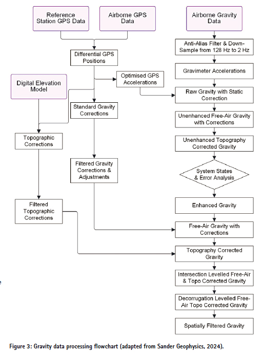
Sander Geophysics’ proprietary software was used for data processing, which involved numerous corrections and f iltering of the observed gravity data. A simplified processing flowchart is shown in Figure 3, illustrating the complexity of the procedure. The airborne GNSS antenna location was determined with an accuracy of better than 5 cm by differentially correcting the airborne GNSS data with respect to the reference stations.
The raw gravity data was corrected for the effects of aircraft acceleration before the standard corrections were applied, i.e. Eötvös correction, normal gravity correction, atmospheric correction, free-air correction, full 3D topographic Bouguer correction, static correction (absolute gravity was established where the static readings were made before and after the f lights so that the relative gravity data could be tied into the national gravity datum) and level correction (based on intersections with tie lines and grid-based de-corrugation). Tidal corrections were not applied, as they are generally not necessary for airborne gravity processing due to their small magnitude. This resulted in determining the free-air anomaly and the Bouguer anomaly (both in mGal).
Simply put, the gravity anomaly indicates the difference of a gravity measurement from the expected value. Depending on the type of correction applied to the observed gravity data at the point of observation, we distinguish between the free-air anomaly (corrected for the height at which it was measured, i.e. reduced to the ellipsoid or geoid) and the Bouguer anomaly (corrected for the height at which it was measured and also the attraction of terrain, i.e. the mass of rock between the measurement point and the ellipsoid or geoid). These anomalies basically show the gravity variation due to the Earth not being quite an ellipsoid/geoid in shape and having variations in density due to the different minerals of which it is made. The free-air gravity anomaly includes all these variations in the shape of the Earth and in the density of the minerals. The Bouguer gravity anomaly removes the signal due to the shape variations and keeps only that due to the density variations, which is most useful for geology and exploration.
Further filtering and gridding followed to reduce noise and generate grids with a 500 m grid size. Firstly, a 70-second, along-track, cosine-tapered low-pass f ilter (equivalent to a 4,200 m filter when accounting for the aircraft’s ground speed of 60 m/s) was selected, and the filtered data was then gridded using a minimum curvature algorithm that averages all values within any given grid cell and interpolates the data between survey lines to produce a smooth grid. In the second filtering stage, low-pass filtering (directly equivalent to spatial averaging) was applied to the grid to achieve better noise reduction than by simply increasing the degree of line filtering. Essentially, the survey area is over-sampled by a line spacing that is smaller than the grid f ilter used. The low-pass filter acts to average data within the radius of its filter dimension, retaining the common signal on adjacent lines and cancelling out random noise. The final data provided a resolution of 2,100 m and 2,500 m, which is expected for the line spacing used (2,250 m onshore and 2,500 m offshore).
Western NSW
Xcalibur Multiphysics was contracted to complete Western NSW, roughly covering the western two thirds of the state (Xcalibur Multiphysics, 2024). The principal survey traverse lines were oriented due north and spaced at 2,000 m, while tie lines were oriented east west at 90º and spaced at 73 km. The survey was flown with a target clearance of 160 m above ground level (following a drape) and a target average ground speed of 65 m/s. Flights commenced in June 2022 and lasted for 14 months, with a total of 413 flights conducted to complete 268,517 line kilometres.
A single-engine Cessna C208B Grand Caravan was used, operating out of Broken Hill, Cobar, Dubbo and Griffith, as well as Yarrawonga, Victoria. Temporary GNSS reference stations were established at each airport and coordinated via Geoscience Australia’s AUSPOS service (GA, 2025), based on datasets of at least 8 hours duration covering the expected time period of an average production flight.
Gravity data was collected with a Falcon Airborne Gravity Gradiometer (AGG) system, which has been optimised for airborne broadband geophysical exploration. The main steps in the Falcon processing flow utilising Xcalibur proprietary software included a dynamic correction (to reduce the effects of aircraft accelerations), demodulation (to transform the accelerometer measurements in the gravimeter from the rotating frame back into a spatial reference frame), self-gradient correction (to account for time-varying gravity gradients caused by the changing heading and attitude of the aircraft during flight), terrain correction (derived from a Digital Terrain Model and using the standard average crustal density of 2.67 g/cm3) and level correction to the regional data using the 2019 Australian National Gravity Grid (ANGG, see Lane et al., 2020).
Once the gradient data channels were fully processed and levelled, noise reduction processing was carried out. The quality (precision) of the Falcon data is measured using the Falcon Difference Noise (the two independent sets of gradiometers inside the instrument allow a noise estimate to be taken at each measurement). The data is acceptable if the noise value is below 5 Eö. However, in this case, for lines where the turbulence was greater than 0.981 m/ s2, the noise limit was increased to 7 Eö.
The noise reduction process is designed to reduce acquisition-related noise by targeting signal response with a linear spatial frequency along the survey line direction. This maximises the resolution of the finished dataset so that it is approximately equal to the line spacing, while also reducing the noise power on the measured data. When the line spacing is smaller than the resolution of the initial signal processing, this process allows for a reduction in noise and increase in resolution. In this case, the line spacing was much larger than the initial signal processing resolution, causing a smaller noise reduction effect but still improving final data quality.
Now that the measured gradients were fully processed, the data was transformed into the components of the gradient tensor. This process uses a Fourier transformation approach to transform the measured tensor components into the full gravity gradient tensor data and the vertical gravity data (Dransfield and Chen, 2019).
The final processing step was the regional conforming process, which corrects the vertical gravity data for very long wavelength errors introduced by the vertical integration of the vertical gravity gradient data. The data was conformed via the Earth Gravitational Model 2008 (EGM2008, see Pavlis et al., 2012), using a filter cut-off wavelength of 200 km, followed by terrain corrections using the standard average crustal density of 2.67 g/cm3.
The conforming process required a significant number of iterations to get an acceptable result as it had never been applied to a survey of such large dimensions before. The standard method had to be revised to ensure the final product met all survey requirements. The approach used was to conform the vertical gravity gradient before the integration. Once this was completed, a second conforming was required to account for very long wavelength integration errors, following the standard methodology but utilising a filter cut-off of 500 km. Considering the line spacing (2,000 m) and the grid size (500 m), the resolution of the final data was determined to be either 1,500 m or 2,000 m.
Quality assurance & final grid production
During and after data acquisition, an independent, third-party subject matter expert checked and verified that the collected data met the quality specifications. Final quality assurance was then performed and the final gridded data products produced (McCubbine, 2024). This ensured that these datasets, captured by two suppliers using different methodologies and equipment, could be integrated into a consistent and reliable set of gravity anomaly grids covering the entire state.
The datasets were evaluated by comparing the point-located and gridded gravity anomaly data to two key reference datasets: the EGM2008 gravity model and the 2019 ANGG. For Eastern NSW, the overall standard deviation of the differences was approximately 2-3 mGal for the comparisons between supplied/recomputed Bouguer anomalies and the ANGG and around 6-7 mGal for the comparison between the geodetic free-air anomaly data and the EGM2008. The Western NSW data also showed high fidelity, with the final gridded datasets exhibiting standard deviations of 1.5 and 1.7 mGal when compared to the ANGG and EGM2008 reference grids, respectively. The higher agreement is due to the Western NSW data undergoing a regional conforming process. These statistics underscore the reliability of the processed datasets for use in regional-scale mapping.
Additional processing was required to ensure consistency across the two datasets. This involved producing a line-by-line levelling adjustment of the Eastern NSW data to align it with an existing state-wide dataset, sampled from the ANGG. This corrected any discrepancies and biases that arose from limitations of the data collection and ensured that the final gridded products accurately reflect the gravity anomalies across NSW. A new point-located data file was reproduced to include the additional levelling corrections and application to the supplied gravity anomalies.
The final data augmentation and gridding process involved the following four steps:
1. Data preparation: The point located data from both suppliers was extracted and block-averaged to half the flight line spacing on a line-by-line basis.
2. Residual calculation: A long wavelength reference signal was subtracted from the gravity anomalies to create a ‘zero-mean’ residual for gridding. The reference signal was derived from a 50 km filtered version of the ANGG data.
3. Gridding: The residuals were interpolated using Least Squares Collocation (LSC), a method that accounts for spatial correlations in the data. This involved f itting the Forsberg (1987) covariance function and solving matrix inversion problems to produce gridded datasets at a 15 arc-second resolution.
4. Restoring long wavelengths: The reference signal was added back to the gridded residuals to produce the final gravity anomaly grids.
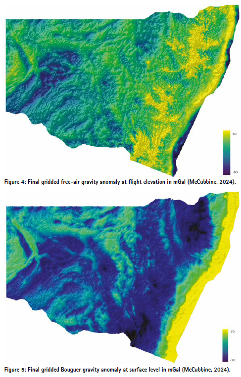
Three final gridded datasets were produced in the GDA2020 at a resolution of 15 arc-seconds (500 m):
• Free-air gravity anomaly at f light elevation (Figure 4).
• Bouguer gravity anomaly at flight elevation.
• Bouguer gravity anomaly downward continued to the topographic surface (Figure 5).
Two surfaces were established as grid nodes to facilitate the interpolation of gravity anomaly data onto a regular grid. The first, a ‘flight-level surface’, was derived by block-averaging the aircraft’s GNSS positioning data into 500 m grid cells, representing the flight elevation grid nodes. The second, a ‘topographic surface’, was constructed by clipping out the relevant area from the 2019 ANGG ellipsoidal Digital Elevation Model, providing a surface-level height reference. The point-located gravity anomaly data was then interpolated onto a 15 arc-second output grid using LSC, ensuring consistency between the reference surfaces and the final gridded product. These gridded gravity datasets provide seamless, coherent maps of the gravity field across NSW. The careful assessment, correction and gridding processes have ensured that these datasets are accurate, reliable and suitable for a wide range of applications.
A state-wide gravity model for NSW
The NSW Gravity Model was delivered on time and within scope and budget due to a collaborative approach between DCS Spatial Services, the Geological Survey of NSW and Geoscience Australia. The collective commitment to enhance the quality of the gravity model by uniting our efforts across state and federal government departments was a strategic decision made to make NSW an easier and more productive place to work, while also supporting national interests. Working closely with experts across different teams allowed us to maximise the collective impact for many diverse applications, delivering the best possible benefit for our customers. As a by-product, we even delivered a gravity model for the ACT, an entirely different jurisdiction – this was much easier than flying around it!
DCS Spatial Services was responsible for managing the project, with Geoscience Australia providing technical expertise and the Geological Survey of NSW met the requirements to deliver a fair playing field for exploration. Gravity datasets are very useful for geodesy and geology, but these two sciences have slightly different requirements. The former needs gravity relative to the geoid, while the latter needs gravity relative to the ellipsoid. Close collaboration ensured that these requirements were met, along with supporting other use cases.
The general public was informed and educated about the data collection flights by DCS Spatial Services via media releases, Frequently Asked Questions and its website (including a video detailing the work to be undertaken). It was stressed that people’s privacy would be protected as the aircraft would only be equipped with an instrument measuring gravity data and not be capable of capturing images of property, infrastructure or individuals. It was also emphasised that these instruments do not emit any signals or impact people, animals or infrastructure and have been used for decades throughout Australia and globally.
Challenges encountered and resolved along the way included delays due to adverse weather conditions or scheduled aircraft maintenance, landholder complaints across Western NSW, access to restricted airspaces, AGG sensor system failure, twin-engine aircraft availability for data acquisition, unaccounted safety audits due to the use of multiple aircraft, optimistic time allocation for data processing, issues related to meeting the contract specifications, and difficulties in the integration and merging of the datasets collected by the two suppliers.
We gratefully acknowledge the collaboration with other state jurisdictions undertaking airborne gravity surveys at the time, which was crucial in enabling the NSW data capture to be completed on time. In particular, Land Use Victoria, the Geological Survey of Victoria and the South Australian government are thanked for providing access to the twin-engine aircraft being used for their gravity surveys.
Data availability & benefits
The gravity data is owned by the NSW Government and freely available to the public via its Spatial Collaboration Portal (DCS Spatial Services, 2025) and the Geological Survey of NSW’s MinView platform (DPIRD, 2025). It is also included in the national geoscience database and accessible via the Geophysical Archive Data Delivery System (GADDS) managed by Geoscience Australia. Making data available in various forms enables it to be used and combined with other sources to generate valuable products for diverse applications. Derived products, such as updated geoid models for GNSS positioning, will be made available in due course.
The NSW Gravity Model positions NSW as a leader in airborne gravity data coverage in Australia. This new dataset will significantly improve the gravity (and gravimetric quasigeoid) model and thus the accuracy of GNSS derived physical heights for a wide range of applications relying on the f low of fluids, such as floodplain management and flood modelling, waterway navigation management, roadway and drainage design, groundwater management, agricultural management, and surveying in general. It will also allow geoscientists to further their understanding of Australia’s geology and how it has evolved over time, and assist in the management of earth resources, infrastructure and natural hazards. Finally, the NSW Gravity Model raises the state to the forefront of potential AVWS early adopters and promotes it as an ideal test area to evaluate any new height datum’s performance and user impact.
Conclusion
This paper has presented the NSW Gravity Model, Australia’s first state wide gravity model produced from a single airborne gravity survey campaign. It has provided some background on airborne gravimetry, introduced the NSW Gravity Model, discussed its data collection and processing, and outlined the benefits this model will provide to the surveying profession and wider community, with gravity data made freely available to the public for the benefit of all.
References
DCS Spatial Services (2025) Spatial Collaboration Portal, https:// portal.spatial.nsw.gov.au/ portal/ (accessed Sep 2025).
DPIRD (2025) MinView, https:// www.resources.nsw.gov.au/ geological-survey/minview (accessed Sep 2025).
Dransfield M.H. and Chen T. (2019) Heli-borne gravity gradiometry in rugged terrain, Geophysical Prospecting, 67(6), 1626-1636.
Fairhead J.D., Cooper G.R.J. and Sander S. (2017) Advances in airborne gravity and magnetics, Proceedings of Exploration’17: Sixth Decennial International Conference on Mineral Exploration, Toronto, Canada, 22-25 October, 113-127.
Featherstone W.E., McCubbine J.C., Brown N.J., Claessens S.J., Filmer M.S. and Kirby J.F. (2018) The first Australian gravimetric quasigeoid model with location-specific uncertainty estimates, Journal of Geodesy, 92(2), 149-168.
Featherstone W.E., McCubbine J.C., Claessens S.J., Belton D. and Brown N.J. (2019) Using AUSGeoid2020 and its error grids in surveying computations, Journal of Spatial Science, 64(3), 363-380.
Forsberg R. (1987) A new covariance model for inertial gravimetry and gradiometry, Journal of Geophysical Research, 92(B2), 1305-1310.
GA (2025) AUSPOS – Online GPS processing service, http://www. ga.gov.au/scientific-topics/ positioning-navigation/geodesy/ auspos (accessed Sep 2025).
Harrison C., Brown N., Dawson J. and Fraser R. (2024) Geocentric Datum of Australia 2020: The f irst Australian datum developed from a rigorous continental-scale adjustment, Journal of Spatial Science, 69(1), 167-179.
ICSM (2021) Australian Vertical Working Surface (AVWS) technical implementation plan, version 1.6, https://www.icsm. gov.au/publications/australian vertical-working-surface technical-implementation plan-v16 (accessed Sep 2025).
Janssen V., Grinter T. and Jansen M. (2025) The NSW Gravity Model: Australia’s first state-wide airborne gravity model, Proceedings of FIG Working Week 2025, Brisbane, Australia, 6-10 April, 19pp.
Janssen V., Haasdyk J. and McElroy S. (2016) CORSnet-NSW: A success story, Proceedings of Association of Public Authority Surveyors Conference (APAS2016), Leura, Australia, 4-6 April, 10-28.
Janssen V. and McElroy S. (2021) The Australian Height Datum turns 50: Past, present & future, Proceedings of APAS Webinar Series 2021 (AWS2021), 24 March – 30 June, 3-27.
Jekeli C. (2003) Statistical analysis of moving-base gravimetry and gravity gradiometry, Report no. 466, Geodetic Science, Ohio State University, Columbus, Ohio.
Kennett B.L.N., Chopping R. and Blewett R. (2018) The Australian continent: A geophysical synthesis, ANU Press & Geoscience Australia, Canberra, 133pp.
Lane R.J.L., Wynne P.E., Poudjom Djomani Y.H., Stratford W.R., Barretto J.A. and Caratori Tontini F. (2020) 2019 Australian National Gravity Grids explanatory notes, https://ecat. ga.gov.au/geonetwork/srv/eng/ catalog.search#/metadata/144233 (accessed Sep 2025).
McCubbine J. (2024) New South Wales statewide gravity anomaly maps from airborne gravimetry data – Processing report: Data assessment, augmentation and grid production, unpublished technical report.
NRCan (2025) CSRS-PPP, https:// webapp.geod.nrcan.gc.ca/ geod/tools-outils/ppp.php (accessed Sep 2025).
Pavlis N.K., Holmes S.A., Kenyon S.C. and Factor J.K. (2012) The development and evaluation of the Earth Gravitational Model 2008 (EGM2008), Journal of Geophysical Research: Solid Earth, 117(B4), B04406.
Preaux S. (2016) Airborne gravity data quality assessment, presented at NGS Airborne Gravity for Geodesy Summer School, Silver Spring, Maryland, 23-27 May, https://www.ngs.noaa.gov/ GRAV-D/2016SummerSchool/ (accessed Sep 2025).
Sander Geophysics (2024) Airborne gravity survey in New South Wales, eastern block, unpublished technical report.
Wooldridge A. (2010) Review of modern airborne gravity focusing on results from GT-1A surveys, First Break, 28(5), 85-92.
Xcalibur Multiphysics (2024) NSW Live Program: NSW Gravity Model – Processing and logistics report, unpublished technical report.


 (76 votes, average: 1.11 out of 5)


Leave your response!