| GNSS | |
Space Weather, from the Sun to the Earth, the key role of GNSS
The goal of this paper is to give a clear view of the Sun Earth relationships that are complex. The phenomena acting at large scales and essentially related to dynamic and electromagnetic physical processes have been addressed. Besides physics, the work done to develop the training in Space Weather by focusing on Global Navigation Satellite Systems has also been presented. We present this paper as a series in two parts. In this issue the focus is on physics of the relationships Sun, Earth
|
 |
|
 |
|
 |
|
 |
|
This paper presents a study made for the Seminar on Space Weather and its effects on GNSS held in conjunction with United Nations/Nepal workshop on the applications of GNSS held in Kathmandu, 6 to 12 December 2016. The Seminar focused on cross-cutting area, in particular resiliency, the ability to depend on space systems and the ability to respond to the impact of events such as adverse space weather.
The aim is to give an outline of the Space Weather and its effects on GNSS receivers, and this in relation to the international organizations in charge of the harmonization of the various GNSS systems. This article is composed of 3 parts: Part I: Physics of the relationships Sun Earth and Meteorology of Space, Part II: GNSS teaching and parameters that can be deduced from GNSS receivers, Part III: Building capacity of developing countries in using GNSS technology for sustainable development
From the Sun to the Earth, Space Weather and its effects
Emissions from the Sun
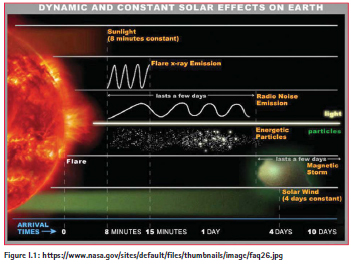
The sun is our star and it influences the terrestrial environment according to different channels, the two main channels are:
1) The radiation channel
2) The particle channel. Figure I.1 shows the different radiations and particles. From the top to the bottom, we have the light, the X-rays and the radio noise emissions. All these phenomena move at the speed of light (300000km / s) and reach the earth in 8 minutes.
After, there are the energetic particles, Magnetic storms and the regular solar wind. For these physical processes, the time to arrive to the Earth depends on their speed, from few 15 minutes for the energetic particles to several days for the regular solar wind.
What is Space Weather and why it is important? The role of ionosphere
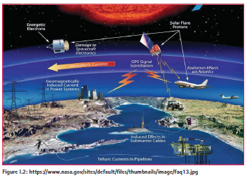
Solar emissions affect the terrestrial electromagnetic environment. Figure I.2 presents some types of perturbations: energetic particles cause damage to satellites and solar radiation affects aviation.
As far as this presentation is concerned, we are more interested in the GNSS signal and thus in the effects of the ionosphere on the GNSS system. The ionosphere is an ionized layer located between 50 and more than 1000 km around the earth. It is the layer of the atmosphere that most disrupts the GNSS signal.
In this layer electric currents circulate (Richmond, 1995). These ionospheric electric currents induce telluric currents in pipeline or submarine cables and can also cause power failure of transformers. Space weather consists to anticipate the action of solar phenomena and try to predict how these phenomena can disrupt all our new technologies (Lilensten and Blelly, 1999; Knipp, 2011)
The Sun and regular connections between the Sun and the Earth
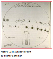
The sun has been observed for several millennia. During the Middle Age, due to the use of the first telescopes by Galileo, the scientists began a study of the sunspots. They have recorded them since about 1611. Figure I.3a shows the motion of a sunspot drawn by Scheiner, Jesuit Father Mathematician working at the University of Ingolstadt (Near Augsburg in Germany). During the Middle Age, scientists did not know what these sunspots were.
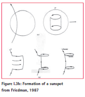
It was only at the beginning of the 20th century that Hale discovered the existence of the poloidal solar magnetic field. At the top left of figure I.3b is presented the poloïdal solar magnetic field. In fact, the sun turns on itself at a different speed between the pole and the equator. About ~27 days at the equator and ~ 31 days at the poles. The differential velocity between the poles and the equator twists the lines of the poloïdal field and creates magnetic loops which are the sunspots. Figure I.3b shows the formation of a sunspot.
The amplitude of the poloidal field is 10 G and the amplitude of the toroidal field (sunspots) is 3-5 kG. The poloidal magnetic field reverses every 11 years (Li et al., 2011). The toroidal magnetic field, sunspot cycle has a period of about 11 years. The two components of the solar magnetic field are anti-correlated. The maximum of the poloidal field occurs at the minimum of the toroidal magnetic field (cycle of spots).
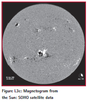
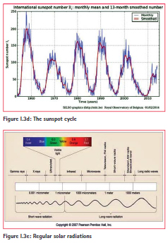
Figure I.3c shows a solar spot observed by the SOHO satellite. Figure I.3d shows the variation of the sunspot cycle over the last 6 decades.
These two components of the solar magnetic field influence the terrestrial environment differently as we shall see later.
The sun is a dynamo which converts motion in electricity.
Figure I.3e shows the complete spectrum of solar radiation from gamma rays to radio waves. In this figure the visible and infrared radiation reaching the ground are presented in color.
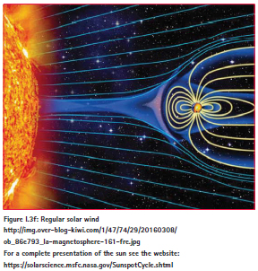
Figure I.3f shows the solar wind, which compresses the magnetosphere (cavity of the earth’s magnetic field), at the front and stretches it at the rear.
The regular solar wind is a constant stream of coronal material that flows off the sun at a speed of ~300-400km/s. It consists of mostly electrons, protons and alpha particles with energies usually between 1.5 and 10 KeV. The Earth’s magnetic field acts as a shield for solar wind. However, there are regions of the ionosphere that are directly connected with the interplanetary medium and this the solar wind flow.
The Earth
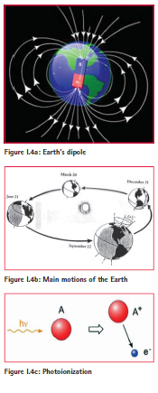
Earth as the sun is a moving magnetic body. Figure I.4a shows the Earth’s magnetic field, which is approximately that of a dipole. Figure I.4b presents the two main movements of our planet which are the rotation on itself and the revolution around the sun. These two movements introduce diurnal and seasonal variability to all the terrestrial phenomena.
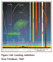
Around the earth, solar radiation, mainly Ultra, Extreme Ultra Violet and X-rays, ionize the atmosphere at altitudes ranging from about 50 km to more than 1000 km. Figure I.4c shows the process of photo ionization. The solar radiation tears an electron from an atom and thus forms an electron ion pair. There is only one ionized atom on 1 million atoms. Figure I.4d shows the radiations which ionize and which do not reach the ground.
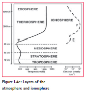
Only the visible and infrared radiations reach the ground. Figure I.4e shows on the left the layers of the atmosphere presented on a scale of temperature (from 300 to 1000°K) and on the right the layers of the Ionosphere presented on a scale of the number of electrons per unit volume. The Ionosphere is located mainly at the level of the atmospheric layer called thermosphere, see books on ionosphere by Rishbeth and Gariott, 1969 and Davies, 1990.
In the section The Sun and regular connections between the Sun and the Earth, we have presented the regular phenomena that connect the sun and the earth, in following sections we will present the perturbations of the sun that can dramatically affect our environment.
Solar flare and solar burst
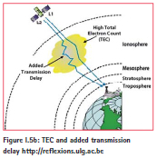
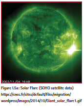
The Solar flare is a significant emission of X-radiation and the solar burst a significant emission of radio noise, see figure I.3e on the spectrum of solar radiation. Figure I.5a shows a solar flare observed by the SOHO satellite in 2003, on November 4. A solar flare creates important additional photo ionization in the ionosphere which affects the GNSS signal and added a transmission delay see figure I.5b.
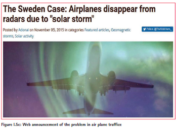
The solar burst is a strong increase in the radio noise of the sun. If the radio frequency emitted by the sun is the same as airport radars, there is a serious incident as the radars can no longer follow the trajectories of the planes. They are saturated by the disturbed radio signal from the sun.
“The 2015 Nov. 4th there is a radio burst [15.30 to 16.30 LT] exceeding everything before. It was so strong that neither GPS nor radar nor communication nor instrument landing system did work properly. All these receivers were completely saturated by the radio radiation, instruments went blind”, figure I.5c, communication from Christian Monstein.
The disturbed solar wind
The solar wind is a flux of particles that regularly escape from the sun. Some events such as coronal mass ejections or fast winds associated with coronal solar holes can disrupt this solar wind and create near-earth disturbances called magnetic storms see figure I.1.
The solar wind carries with it a part of the solar magnetic field which is called interplanetary magnetic field IMF. This magnetic field acts as a trigger for magnetic storms. If it is directed southward, in the opposite direction to the terrestrial magnetic field, there is reconnection of the interplanetary magnetic field and the terrestrial magnetic field (Dungey, 1961). The magnetosphere is open and is completely under the influence of the solar wind. There is a magnetic storm.
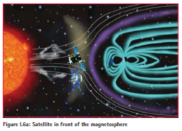
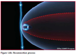
Figure I.6a shows a satellite which is located in front of the magnetosphere and which makes it possible to know the arrival of a solar wind that can generate strong magnetic storm. Figure I.6b shows the favorable conditions for the triggering of a magnetic storm, that is to say an interplanetary magnetic field directed towards the South.
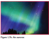
The auroral zone
As mentioned earlier, the earth’s magnetic field (magnetosphere) acts as a shield and protects the earth from particles from the solar wind. However, there exists near the poles a region where the solar particles can penetrate directly, it is the polar cusp. There is also a region around the pole where the particles precipitate and create an extra ionization which is not due to solar radiation but to particles of the solar wind.
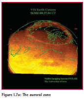
Figure I.7a shows a light circle around the pole that corresponds to the auroral zone, where the particles precipitate. It is in this region that one can observe auroras (borealis aurora for the northern and austral aurora for southern hemisphere). The particles excite the atoms that emit light and create aurorae (Figure I.b).
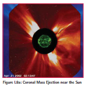
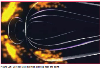
The Coronal Mass Ejection: CME
Billions of tons of coronal matter are ejected from the sun and head towards the earth. If the magnetic field transported by the CME is directed towards the south, there is a magnetic storm. In general, coronal mass ejections are preceded by solar flares and associated with interplanetary shock. The Solar Flare arrives in 8 minutes on Earth while Coronal Mass Ejection takes 1 or more days depending on its speed.
Figure I.8a shows a CME seen by the SOHO satellite. One distinguishes the coronal matt er ejected from the sun. Figure I.8b shows the arrival of the CME near the earth, this figure is an artistic view. If the magnetic field carried by the CME is directed southward and therefore opposite to the earth’s magnetic field, there is a magnetic storm. The occurrence of CME is related to the sunspot cycle. There is much more CME at the maximum of the sunspot cycle (toroïdal component of the solar magnetic field).
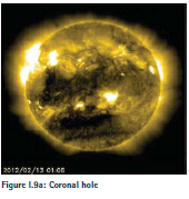
High Speed Solar Wind Stream
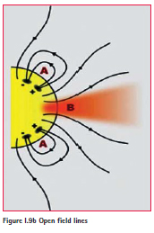
As we have seen previously, there is a compon ent of the poloidal solar magnetic field which has open field lines on the interplanetary space allowing rapid solar wind to escape from these structures called coronal holes
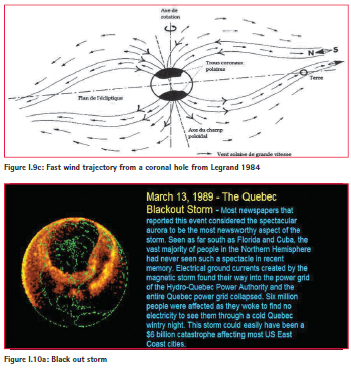
Figure I.9a shows a coronal hole observed by the SOHO satellite, this hole presents itself as a large black spot on the sun. Figure I.9b shows the lines of the poloïdal solar magnetic field open on the interplanetary medium. If the Earth is on the trajectory of a fast solar wind carrying an IMF interplanetary magnetic field directed towards the south, there is a magnetic storm (see figure I.9c). There is a maximum occurrence of fast winds during the decay and minimum phase of the sunspot cycle, so that the poloidal magnetic field grows to its maximum.
Telluric induced currents
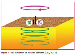
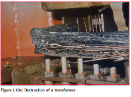
The currents induced in the Earth by the electric currents circulating in the ionosphere strongly disturbed the Earth’s environment. During strong magnetic storms, the auroral oval descends towards the mid-latitudes (see figure I.10a) and as a consequence the strong auroral electric currents will induce telluric currents at the middle latitudes or even the low latitudes (figure I.10b) and produce electrical failures in the transformers and cut down the electricity (figure I.10c). This was the case during the storm of 13 March 1989
St Patrick’s Day magnetic storm: impact on a CME on the ionospheric ionization
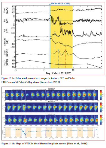
Figure I.11a illustrates the variations of different parameters during the magnetic storm of St Patrick’s Day (March, 17, 2015). From the top to the bottom, there are the solar wind in km/s, the Bz component of the IMF (in nT) , the magnetic index Ae (in nT) which is related to the ionospheric currents in the auroral zone, the magnetic index SYM-H (in nT) related to the electric currents, in the magnetosphere (Mayaud, 1980; Menvielle and Berthelier, 1991; Amory-Mazaudier, 2010), the Global TEC and the solar index F10.7cm related to the solar radiation.
At the arrival of the CME on March 17, there is a large increase of the solar wind speed associated to a southward component Bz of the IMF; these two conditions are favorable for the development of a magnetic storm. (see section: the disturbed solar wind).
Figure I.11a shows two large increases of the Global Electron Content (GEC) occurring after increases of the Ae magnetic index (auroral currents) and large decreases of SYM-H (magnetospheric equatorial current). These large increases o the GEC are followed by large decreases of GEC.
Figure I.11b shows the TEC maps obtained from 200 GPS stations. We have presented these maps for the 3 sectors of longitude: Asian, African and American, for the period March 14 to April 1st 2015. The x-axis represents the magnetic latitudes with the magnetic equator at zero. The y-axis represents time. On March 17 at 04.45 UT, a CME hits the magnetosphere. This CME was emitt ed by the sun, 2 days earlier, on March 15. Before the arrival of the CME, on March 14, 15 and 16, we observe on the VTEC maps the signature of the equatorial fountain consisting of 2 VTEC maximum at 15° North and 15° South of the magnetic equator. The impact of CME is very diff erent depending on the sector of longitude considered. In the Asian longitude sector, there is a total disappearance of the ionosphere on 18 March. In the American longitude sector, there was a marked increase in ionization on 17 March. In the African sector, the impact is lower. At the bott om of the figure there is the H-SYM magnetic index which illustrates the variation of magnetospheric currents during the magnetic storm.
Scintillations
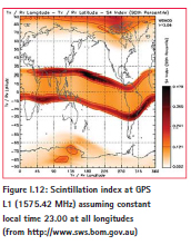
Ionospheric scintillation is the rapid modification of radio waves caused by small scale structures in the ionosphere.
Ionospheric scintillation is primarily an equatorial and high-latitude ionospheric phenomenon, although it can (and does) occur at lower intensity at all latitudes.
Ionospheric scintillation generally peaks in the sub-equatorial anomaly regions, located on average ~15° either side of the geomagnetic equator.
Ionospheric scintillations are one of the major problems of GNSS propagation in the equatorial zone. They are not due to solar events such as coronal mass ejections or fast winds associated with coronal solar holes, there are related to Instabilities in the ionospheric Plasma, see the book Kelley(1989) on equatorial ionosphere.
Concluding remarks
In this part we have presented the dominant physical processes of the space weather, without which there is no space weather. These dominant physical processes are:
– the magnetic fields and the motions of the Sun and the Earth,
– the magnetosphere, the Ionosphere, the auroral zone,
– the more common solar disturbances due to extra radiations: solar flare, solar burst,
– the coronal Mass Ejection and High speed solar wind related to coronal hole, at the origin of magnetic storms,
– The ionospheric scintillations, related to ionospheric plasma instabilities.
But, there are many other secondary physical processes that also influence the space weather.
In short the space weather is the science of the dynamic and electromagnetic interactions of two magnetic bodies in motion: the sun and the Earth.
This new science includes two aspects: 1) the physics of Sun Earth relations and 2) the effects of solar disturbances on new technologies.
In this paper we will focus in the second part on the GNSS technology. In order to make progress in space meteorology there is the need for international interdisciplinary cooperation. This is the mission of the International Space Weather Initiative (ISWI: http://www.iswi-secretariat.org).
This network promotes a synthetic training on Sun-Earth Relationships. This training is given in schools in the different countries over the world.
This network is based on different rules:
– Distribution of scientific instruments in countries where instruments are lacking,
– The training of students over the world and particularly in developing countries,
– The supervision of PhD, and capacity building in Space Weather, particularly in developing countries,
– Public conferences on Space Weather for public science.
Some students trained in this network defended PhD connecting the recent discoveries of the physics of the sun to the ionosphere (Ouattara, 1999; Zerbo, 2012)
The websites with the data concerning this part are: ISGI http://isgi.unistra.fr/ geomagnetic_indices.php
Institut Royal Météorologique de Belgique http://aeronmie.be International Association of Geomagnetism and Aeronomy IAGA https://www.ngdc.noaa.gov/IAGA/vdat/
NASA SOLAR SCIENCE http:// solarscience.msfc.nasa.gov/
NASA SOLAR DATA https://igscb.jpl. nasa.gov/igscb/data/format/rinex211.txt
NOAA ftp://ftp.swpc.noaa.gov/ pub/weekly/Predict.txt
OMNIWEB : http://omniweb. gsfc.nasa.gov/
Satellite ACE http://www. swpc.noaa.gov/ace
Satellite SOHO http://sohowww. nascom.nasa.gov/
Site web Space Weather http:// spaceweather.com/
Bibliography
Amory-Mazaudier, C,(2010), Electric Current Systems in the Earth’s Environment, Nigerian Journal of Space Research, Deutchetz Publishers, Vol. 8 ISSN 0794-4489, pages 178-255.
Azzouzi I., Y Migoya-Orué, C. Amory Mazaudier, R Fleury, S M Radicella, A Touzani, (2015), Signatures of solar event at middle and low latitudes in the Europe-African sector, during geomagnetic storms, October 2013, Advances in Space Research, doi: http:// dx.doi.org/10.1016/j.asr.2015.06.010
Friedman, H., 1986. Sun and Earth, Scientific American Library, An imprint of Scientific American Books, lnc., 251p.
Davies K., (1990) Ionospheric radio, Peter Peregrinus Ltd., ISBN 0-86341-186-X.
Dungey, J.W.,(1961), Interplanetary Magnetic field and the auroral zone, Phys. Rev., 7, 47-49.
Kelley, M.C., (1989), the Earth Ionosphere, ed. Academic Press, San Diego.
Knipp, D.J. , (2011), Understanding Space Weather and the Physics behind it, publisher Mc Graw-Hill Education Europe, ISBN 10:0073408905.
Lilensten, J.,P-L. Blelly, (1999), Du Soleil à la Terre, Aéronomie et météorologie de l’espace, Presses Universitaires ,Collection Grenoble Sciences, Université Joseph Fourier Grenoble I, ISBN 9782868834676.
Legrand, J.P.,(1984). Introduction élémentaire à la physique cosmique et à la physique des relations soleil-terre, Editeur Territoire des terres australes et antarctiques françaises, Paris, 308p. Li , Y., J.G. Luhmann, B.J. Lynch and E.K.J. Kilpua ., (2011). Cyclic Reversal of Magnetic Cloud Poloidal Field, Solar Phys. Doi: 10.1007/s11207-011-9722-9.
Luu Viet Hung,(2011) Etude du champ électromagnétique et interprétation des données magnétotelluriques au Vietnam, PhD, 21 décembre, Univ. Paris Sud 11, France.
Mayaud, P.N., (1980) Derivation, Meaning and Use of Geomagnetic Indices, Geophysical Monograph 22, Am. Geophys. Union,Washington D.C.
Menvielle M. and A. Berthelier.,(1991). The K-derived planetary indices: description and availability, Rev. Geophys. 29, 3, 415-432.
Nava, B., J. Rodríguez-Zuluaga, K. Alazo-Cuartas, A. Kashcheyev, Y. Migoya-Orué, S.M. Radicella, C.Amory- Mazaudier, R. Fleury, (2016) “Middle and low latitude ionosphere response to 2015 St. Patrick’s Day geomagnetic storm” J. Geophys. Res. Space Physics, 121, doi:10.1002/2015JA022299.
Ouattara, F., (2009) Contribution à l’étude des relations entre les deux composantes du champ magnétique olaire et l’ionosphère équatoriale, PhD dissertation (Thèse d’Etat), Université Cheikh Anta Diop, Dakar, 3 Octobre 2009.
Richmond,A.,(1995). Ionospheric Electrodynamics, Hanbook of Atmospheric Electrodynamics, Vol II, Chapter 9, 249-280, Edited by Hans Volland. Rishbeth, H., O.K. Gariott (1969), Introduction to Ionospheric Physics International Geophys. Ser., 14 Ed Academic Press, pp 344, ISBN 0125889402, book.
Zerbo, J-L., (2012). Activité solaire, vent solaire, géomagnétisme et ionosphère équatoriale. PhD dissertation (Thèse), Université de Ouagadougou, le 20 Octobre
Watch out for March issue for GNSS training and capacity building.


 (3 votes, average: 3.67 out of 5)


Leave your response!