| Navigation | |
Improved algorithms for sailing calculations
This paper presents new algorithms for rhumbline sailing (RLS) and great elliptic sailing (GES)calculations for route planning and portrayal of navigational paths on Electronic Chart Systems |
|
From the early days of the development of basic navigational software built into satellite navigational receivers, it has been noted that for the sake of simplicity and a number of other reasons, this navigational software is often based on methods of limited accuracy [1]. It is surprising that even nowadays the use of navigational software is still used in a loose manner, sometimes ignoring basic principles and adopting oversimplified assumptions and errors such as the wrong mixture of spherical and ellipsoidal calculations in different steps of the solution of a particular sailing problem [2]. The lack of official standardization on both the “accuracy required” and the equivalent “methods employed”, in conjunction to the “black box solutions” provided by GNSS navigational receivers and navigational systems (ECDIS and ECS) suggest the necessity of a thorough examination of the issue of sailing calculations for navigational systems and GNSS receivers [3].
New formulas have been derived for both Rhumb Line Sailing (RLS) on the ellipsoid and Great Elliptic Sailing (GES). The RLS formulas result from the analysis of the geometry of the loxodrome on the ellipsoid and are simpler and faster than those traditionally used for RLS on the ellipsoid, which are normally based on the Mercator projection formulas. The proposed new algorithm for Great Elliptic Sailing (GES), provides extremely high accuracies comparable to those obtained by the computations of geodesics. Numerical tests show that discrepancies in the computed distances between “geodesic” and “great elliptic arc” are practically negligible for navigation [4].
Rhumbline Sailing (RLS )
The proposed formulas for rhumbline sailing calculations on the ellipsoid solve both the direct and the inverse RLS problem. In traditional navigation the navigator is interested only in the inverse RLS problem that solves for the “course to steer” and the “sailing distance” from one location to another.
In contemporary navigational systems (ECDIS, ECS) the accurate solution of the direct RLS is required for the portrayal of the RLS paths on the displayed electronic chart. The RLS paths (loxodromes) are depicted on the electronic chart through the calculation of the coordinates of intermediate points between the points of departure and destination for specific distance intervals and for a given steering course.
Inverse RLS problem
This section of the algorithm consists of three parts:
Part 1: Calculation of Meridian distance
The calculation of the length of the arc of the meridian is a prerequisite not only for RLS calculations, but also for “geodesic sailing” and “great elliptic sailing”. The fundamental equation for the calculation of the length of the meridian arc on the ellipsoid (figure 1), is:

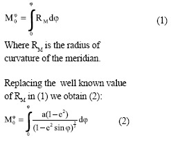
Formula 2 can be transformed into an elliptic integral of the second type, which cannot be evaluated in a “closed” form. The calculation can be performed either by numerical integration methods, such as Simpson’s rule, or by the binomial expansion of the denominator to rapidly converging series, retention of a few terms and further integration by parts. Simpson’s numerical integration does not provide satisfactory results and consequently the methods used are based on the series expansion formulas [5], [6]. The series expansion formulas have the general form of equation (3).
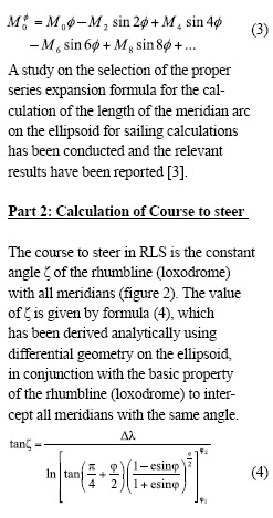

![]()
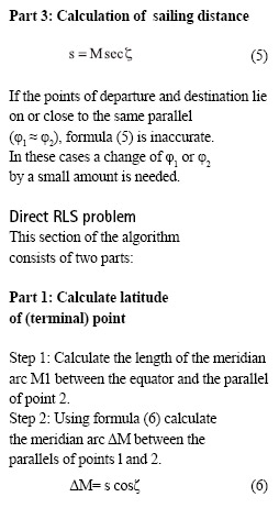
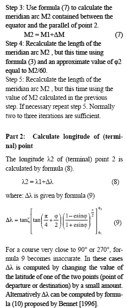
Where, φm is the mean latitude of the points of departure and destination. Formula 9 is derived directly from formula [4] and is simpler than other formulas based on the use of isometric latitude [Bowring 1985, Bennet 1996] and the general formulas of the Mercator projection [Snyder 1987].
Great Elliptic Sailing (GES)
In traditional navigation, the calculation of the elements of the shortest navigation path between two points on the surface of the Earth is usually conducted by the use of a spherical model of the earth and the assumption that the length of one minute arc of any great circle is equal to one international nautical mile. It is obvious that more accurate results can be obtained by the adoption of an ellipsoidal model of the earth and the calculation of the geodesic distances and azimuths. The discrepancies between the results of shortest navigational path calculations on the spherical model of the earth as great circle arcs and on the ellipsoidal model as geodesics, are in the order of 0.27% according to Tobler [7] and in the order of 0.5% according to Earle [2]. In reality and for long distances these discrepancies can exceed 15 nautical miles (about 28.5 km). An example of such a discrepancy is shown through the calculation of the shortest navigational distance from a departure location on the east coast of Australia, such as the entrance of Sydney harbor (φ: 33º 46´.21 S, λ: 151º 31´.964 E) to a destination point on the west coast of South America such as the approaches to Valparaiso in Chile (φ: 32º 59´.998 S, λ: 71º 36´.675 W). The calculation of this distance on the spherical earth model with the above mentioned assumption yields a distance of 6113 nautical miles. The calculation of the same distance on the WGS-84 ellipsoid with very accurate geodetic methods of sub meter accuracy as Vicenty’s [7], yields 6128.4 nautical miles. For this example the difference in calculated distances on the spherical model from those on the ellipsoid is more than15 nautical miles (~28.5 km). The great ellipse is the line of intersection of the surface of the ellipsoid with the plan passing through its geometric center O and the departure and destination points P1 and P2 (figure 3).

For surface navigation applications the great elliptic arc P1P2 approximates very closely the geodesic line and even for the longest possible navigational paths the discrepancies between “geodesic” and “great elliptic arc” are practically negligible. In practice very accurate results can be obtained through the execution of the calculations on the great ellipse rather than on the geodesic [8].
The algorithm starts with the calculation of the eccentricity of the great ellipse and the “geocentric” and “geodetic” great elliptic angles (figure 4) of the points of departure and destination. This part of the algorithm consists of the formulas proposed by Williams [9] because they are simple and straight forward and provide accurate results [4].

For the calculation of the length of the great elliptic the algorithm uses the standard geodetic series expansion formulas for the length of the meridian arc, after their proper modification for the great ellipse by the substitution of the “eccentricity of the ellipsoid” and the “geodetic and geocentric latitudes” with the “eccentricity of the great ellipse” and the “geodetic and geocentric great elliptic angles”. For the calculation of the initial and final course the algorithm adopts the methodology proposed by Bowring [10]. Initially the forward and backward azimuths are calculated on the auxiliary unit sphere as in the classical spherical earth model use in traditional navigation. Then the calculated spherical azimuths are reduced to their ellipsoidal values for the great elliptic arc. These parameters are required for the subsequent calculation of the geodetic coordinates of the intermediate points along the great elliptic arc. The calculation of the geodetic coordinates of the intermediate points along the great elliptic arc is conducted by successive solutions of the direct great elliptic problem using the formulas proposed by Bowring [10].In these successive calculations, in order to avoid propagation of errors, the initial point is always the point of departure and the destination point is the intermediate point concerned. The known parameters in these direct problem solutions are: “the geodetic coordinates of the point of departure”, “the calculated initial course at this point” and “the distance of the intermediate point from the point of departure”. The full set of the formulas used in the algorithm can be found in [4].
Pages: 1 2


 (No Ratings Yet)


Leave your response!