| GNSS | |
Comparison of orthometric heights determined by GPS and simple geometric levelling
The paper develops regression models for the variation of these height differences as function of change in altitude and baseline length |
 |
|
 |
|
 |
|
 |
|
GPS positioning system is designed to determine the position of a point any time and at any place with an accuracy that could reach a few millimeters depending on the type of equipment and the used methodology. In this context, Permanent GPS stations were used to detect displacement of a few mm/year along the Alps (Caporali A. et al., 2000).
The use of GPS technology has evolved rapidly especially in the fields of geodetic sciences and surveying engineering. Nowadays, space technology is witnessing a great revolution in terms of positioning. All Geodetic networks are established using GPS technology, as it is a reliable and efficient mean for geodetic network densification.
If GPS has shown its effectiveness in the planimetric determination, the height positioning remains not demonstrated.
Several studies have experimented the use of GPS for height determination. For example, GPS has been used for the assessment of height variations around the Mediterranean and Black Seas (Becker et al., 2002). GPS combined with a gravimetric geoid have also been used for deriving orthometric heights in North Algeria by Ben Ahmed Daho (2003). In addition, there are many other related studies that have discussed the use of GPS for the purpose of height determination. We can mention Dodson (1995); Dursun et al. (2002); Stig- Coran (2002); Battaglia et al. (2003); Lin (2013); Xingsheng (2013); Cakir et al., (2014); and Peter (2014).
Objectives
Morocco knows the development of a large number of construction sites and arts structure, such as bridges, roads and highways. Engineers in Surveying should connect these structures to the Moroccan General Levelling Network (MGLN). Unfortunately, levelling benchmarks of the MGLN are not available everywhere. Sometimes, surveyors do have to cross several kilometers by geometric levelling to achieve these levelling benchmarks. Such work takes long time and needs great efforts.
For that purpose, surveyors want to know how far they could use GPS instead of geometric levelling to determine orthometric heights from levelling benchmarks that are several kilometers far away from their sites.
In order to respond to surveyors’ preoccupations, we purpose in this article to compare the orthometric heights determined by GPS dual frequency to those obtained by simple geometric levelling. The comparison is discussed with respect to three factors: baseline length, altitude change, and the topography of terrain.
Accordingly, the objectives of this study concern two aspects: First aspect: experimental studies This aspect concerns several experimentations consisting in:
• Use dual frequency receivers to determine the orthometric heights
for a set of known benchmarks of the MGLN and a series of new points, taking in consideration the three factors cited above.
• Measure the orthometric heights of the same set of benchmarks and the new points using simple geometric leveling.
• Compare the heights determined by GPS to those obtained by SGL, the later ones will be taken as reference.
Second aspect: statistical analysis and modeling
This second aspect concerns statistical analysis on the experiments, namely
• Statistically analyze the variation of differences between the two aforementioned height determinations.
• Develop linear regression models expressing the variation of these differences as a function of the baseline length, and the change in altitude, taking into account each type of terrain.
Experimental studies
Basic data
The Department of the National Agency of land registration, Cadastre and Cartography (ANCFCC), has placed coordinates of points as well as data on the MGLN at our disposal. Benchmark files contain approximate coordinates, orthometric heights, and synoptic description, in addition to the approximate distances between benchmarks.
Data collection
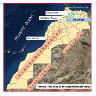
This phase consists in selecting sites of experimentations and collecting data concerning benchmarks and reference points as well. Therefore, we choose three different cases of terrain, corresponding to four different sites in Morocco (see annexe). The corresponding leveling sections are :
• The first case of terrain contains the two axes of Rabat to Temara (northwest of Morocco) and Ait Melloul to Tiznit (south of Morocco).
• The second case of terrain is the axis of Meknes to El Hajeb (middle of Morocco).
• The third case of terrain concerns the axis from Fes to Taounate (North of Morocco).
After that, we draw a rough outline that includes the following elements:
• Choosing some benchmarks of the MGNL: these are chosen so that they are easily accessible, stationnables and clear to facilitate observations of geometric leveling,
• Verification of the existence and status of these benchmarks,
• Choosing new points around these benchmarks. These new points are selected so as to have different baseline lengths and various changes in altitudes with respect to benchmarks. These new points are materialized in stable places with iron.
• Planning GPS mission: determining the observation periods, the number of available satellites, the PDOP, the number of sessions of observation per day, the duration of each session, and establishing a program of GPS observations
Observation campaigns
Before starting observations, we made a check of the homogeneity of benchmarks: this check consisted in determining the changes in altitudes between benchmarks and compare them to the known altitudes. So for the three cases of terrain, the homogeneity tests show that differences between the known altitudes and observed altitudes vary between 0.1 cm and 11.9 cm. adopting a tolerance of 15 cm, we can conclude that benchmarks are homogeneous and stable with respect to each others, therefore they can be used as control points in our experiments.
Note that our GPS Observations are done during several days, for the three cases of terrain. During these experiments, we used only dual frequency receivers of three types. The static mode is used for the control points, (observation time varies from 1 Hour to 4 Hours), while the rapid static mode is used for the new points (minimum of 30 minutes of observations).
Concerning the geometric levelling operations, we used an optical level and a rod graduated in centimeters.
Experiments for the first case study: sites of Rabat-Témara and Sidi Bibi
The first case concerns two sites of flat terrain, the site of Rabat-Temara in north west of Morocco, and the site of Sidi Bibi in the south of Morocco. For these two sites, the lengths of baselines vary from 92 m to 7.6 km.
The first site (Rabat-Temara) is located between the city of Rabat and Temara. On this site, we conducted two sessions of observation, with three fixed benchmarks and seven new points. For this site the altitudes of points vary between 15 m and 54 m, while changes in altitude range from 41 cm to 32.99 m.
The second site of Sidi Bibi is located 22 km south of the city of Agadir. In this experiment, we choose five control points, and ten new points. In this case, we conducted two sessions of observations.
For this second site, the altitudes of points vary between 50 m and 67 m, while the maximum height difference is 16.9 m.
Experiments for the second case study: site of El Hajeb
The second experiment case study concerns the axis Boufekrane-El Hajeb. It is located 18 km south of the city of Meknes. For this second case, the altitudes of points vary between 708 m and 1107 m, with an average altitude of 842 m. Changes in altitudes vary between 31 cm and 394 meters. Distances between selected control points vary from 3 km to 5 km. The maximum baseline length between benchmarks is 15.8 km. For this experimentation, we planned three sessions of GPS observations.
Experiments for third case study: site of Taounate
This site is located along the main road from Fès to Taounate. The average altitude of the levelling points is 407 m, with a minimum altitude of 320 m and a maximum of 465 m.
For this site, we have accomplished a single session of observations with the following data:
• Changes in altitudes vary between 20 cm and 144.99 m, the average is 70 m.
• There are nine new selected points, and three control points.
• Baselines lengths vary between 17 m and 7.6 km.
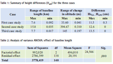
Presentation of results: summary of height differences (GPS vs levelling) for the three cases
After treating the GPS data, and simple geometric leveling, we calculate differences between the orthometric heights (we will use the term height differences) determined by these two technics (GPS and simple geometric leveling). Table 1 summarizes the differences obtained for the three cases of terrain, as well as orthometric heights and baseline lengths for each case.
Referring to this table, we can notice that:
• The differences between GPS orthometric heights and levelling vary between 0 and 13.5 for the three cases.
• We can see that differences vary depending on the baseline length and the altitude change for the three cases.
• Through the obtained results for the three types of terrain, we realize that the orthometric height determination by GPS may depend mainly on two factors, the length of baseline and the change in altitude between the observed points.
• For this purpose, we will carry out a statistical analysis to assess the effect of these two parameters and try to model this variation by considering each type of terrain.
Statistical analysis
In this statistical analysis, we suggest studying the variation of height differences case by case, as follows:
• Effect of baseline length on the determination of height differences (HSGL – HGPS).
• Effect of change in altitude on the determination of height differences (HSGL – HGPS).
• Effect of the type of terrain on the determination of height differences (HSGL-HGPS).
Analysis of variance
Analysis of variance, or ANOVA, was used by SIR Ficher (Dagnelie, 2011), to analyze data from experiments. This test consists in testing the effect of any parameter; by comparing the value of probability Sig at a level of significance. This probability is computed based on the sum of the squares of the differences; the degree of freedom (df); the mean square; and the random variable of Fisher (F). The significance levels are as follows:
• Sig > 0.05 indicates that the test is not significant.
• Sig < 0.05 indicates that the test is significant.
• Sig < 0.01 indicates that the test is highly significant.
• Sig < 0.001 indicates that the test is extremely significant
Analysis of the effect of baseline length
In order to perform this analysis, we gather all obtained height differences (Hdiff) from all the three cases, then, we classify the baselines lengths in 3 classes which are defined for this analysis as follows:
• Class I (short baseline): D < 1 km. For this class, there are 47 cases
• Class II (medium baseline): 1 km < D < 5km. This class contains 46 cases
• Class III (long baseline): 5km < D < 16km. This class includes 48 cases The result of the analysis of variance for the baseline length effect is shown in table 2.
This test (Sig < 0.001) statistically shows that there is a very highly significant effect of baseline length on the orthometric difference (HSGL – HGPS). This means that this difference is very highly dependent on the baseline length.
Test of NEWMAN and KEULS This test procedure compares all pairs of averages at a defined α (5%) level of significance. Thus, it indicates what averages are significantly different from others. We have used this test to compare averages of three classes of baselines. We came up to the following result: The effect of the first class with an average equal to 3.1 is statistically different from the other two classes. The other two classes are statistically identical. From this test, we conclude the following:
• For short baselines (less than one km), height differences (Hdiff) between leveling and GPS gives an average of 3.1 cm.
• For the other two classes, the test shows that the results can be shown as similar. The average height differences (Hdiff) are 8.1 cm for the 2nd class (higher or equal to 1 km and less than 5 km), and 9.1 cm for the 3rd class (higher or equal to 5 km, less than 16 km).
Analysis of the effect of change in altitude
To prepare this analysis, we have grouped all observations, and we have classified the changes in altitudes into 3 classes:
• Class1: Small change in altitude: DH < 10 m. There are 45 cases.
• Class 2: medium change in altitude: 10 m < DH < 100 m. There are 63 cases.
• Class 3: high change in altitude: 100 m < DH < 400 m. There are 33 cases.
The results of the analysis of variances are shown in table 3. This test (Sig < 0.001) shows, that there is a very highly significant effect of change in altitude on the height differences between GPS and leveling.
NEWMAN and KEULS test
Using this test, we compared the averages of the three classes of changes in altitudes, we have achieved the following results.
• The effect of the three classes is statistically different from one class to another
• This difference increases more rapidly with the change in altitude compared to the effect of the baseline length.
For each class of change in altitude, we have obtained the following averages:
• 3.2 cm for the first class (small change in altitude).
• 7.3 cm for the second class.
• 10.7 cm for the third class.
Analysis of the effect of the type of terrain Looking through the results, we note that the height differences between GPS and levelling for the same baseline length and elevation differs from one type of terrain to another. Therefore, we plan to study the influence of the terrain according to the three cases studied. The analysis of variance gives the results as mentioned in table 4.
The ANOVA test shows that the terrain has a very highly significant effect (Sig < 0.001) on the orthometric height differences (Hdiff). Concerning the influence of the terrain, we can conclude that:
• For the first case of terrain, the average of the height difference is 5 cm.
• For the second case of terrain, the average of the height difference is 6.7 cm.
• For the third case of terrain, the average of the height difference is 10.8 cm.
Modelling the orthometric height differences (Hdiff) using linear regression model
Linear regression is an approach for modeling the relationship between a scalar variable Y (dependent variable) and one or more explanatory variables (independent variables) denoted X. The case of one explanatory variable is called simple linear regression. For more than one explanatory variable, the process is called multiple linear regression (Dagnelie, 2011).
In order to study the influence of the change in altitude on the one hand, and the effect of baselines lengths, on the height differences (Hdiff), on the other hand, we use a linear regression model with a single variable. This model has the following form:
Y = Hdiff =a + b X
In this model, we have: Hdiff: represents the height difference between levelling and GPS. X is the random variable, for this study it represents either the change in altitude or the baseline length. a is a constant term b is the regression coefflcient
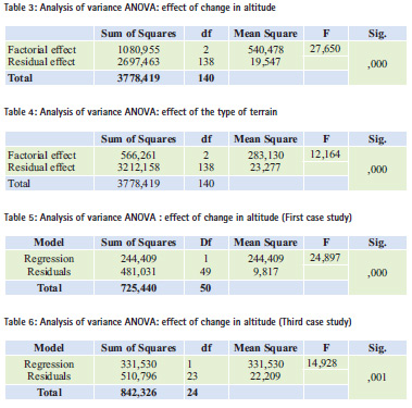
Modelling the orthometric height differences (Hdiff) as function of change in altitude
By studying each case of terrain, we have used a simple regression model to express the relationship between the height difference (Hdiff) and the change in altitude.
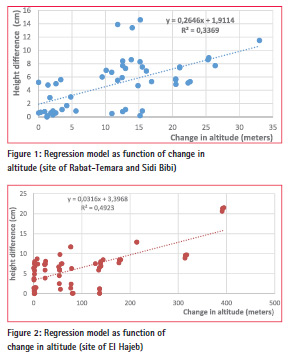
a) The first case study (Rabat- Temara and Sidi Bibi sites)
After regrouping all the height differences (Hdiff) for this case of terrain, the linear regression model can be expressed by the following equation:
Hdiff (cm) = 1.9 (cm) + 0.265
* altitude change (m)
For this model, the height difference will increase by 2.65 cm per 10 m change in altitude, with a constant term of 1.9 cm (figure 1).
The ANOVA test is very highly significant; implying that here is a very highly significant effect of altitude change on height differences (Hdiff) (table 5).
b) The second case study (site of El Hajeb):
The regression model expressing the height difference for this second case of terrain is given by the following equation:
Hdiff (cm) = 3.4 (cm) + 0.032
* altitude change (m) For this second model each altitude change of 100 m, will give a height difference of 3.2 cm, with a constant term of 3.4 cm (figure 2).
c) The third case study (site of Taounate).
Table 6 represents the results of the influence of altitude change on height difference for the third case study.
The ANOVA test is very highly significant, implying that there is a very highly significant effect of altitude change on height differences (Hdiff). This height difference is represented according to the change in altitude by the following model:
Hdiff (cm) = 7.3 cm + 0.076
* altitude change (m)
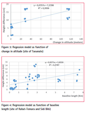
This model displays that the height difference will increase by 7.6 cm for each altitude change of 100 m, with a constant term of 7.3 cm (figure 3) Modelling the orthometric height differences (Hdiff) as function of the baseline length By studying the variation of height differences (Hdiff) as function of baselines lengths, we can use the simple regression model to express the relationships for each study case.
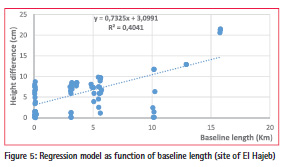
a) The first case study
The coefficients of the regression model for this terrain are represented by the following equation (Figure 4):
Hdiff (cm) = 2.8 + 0.927
* baseline length (Km)
For this case, the height difference, increases by 0.92 cm, for a baseline of 1 km, with a constant term of 2.8 cm.
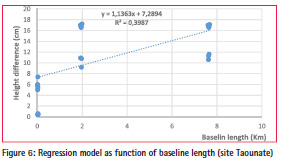
b) The second case study
The coefficients of the simple regression function for this second site are:
Hdiff (cm) = 3.1 cm + 0.732
* length of baseline (km)
For this type of terrain, the height difference increases by 0.73 cm for a baseline of 1 km, with a constant term of 3.1 cm (figure 5).
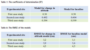
c) The third case study
In this case the ANOVA test is very highly significant. Therefore, the height difference as a function of baseline length can be represented by the following regression equation (Figure 6):
Hdiff (cm) = 7.3 cm + 1,136
* baseline length (km)
This equation shows that the height difference increases by 1.14 cm for a baseline of 1 km, with a constant term of 7.3 cm.
Analysing and assessing the models
in this statistical section, we have developed linear mathematical models that express the variation of height differences (Hdiff) depending on the altitude change on one hand and on the baseline length on the other hand. These Mathematical models show that:
– Regarding to the effect of altitude change, the constant terms of these equations are 1.9 cm, 3.4 and 7.3 cm respectively for the three types of terrains.
– Concerning the baseline length, the constant terms are 2.8 cm, 3.1 cm and 7.3 cm for each case study respectively.
In order to evaluate the performance of these models, we have used two statistical elements: the coefficient of determination (R2) and the RMSE.
The coefficient of determination (R2):
For each model, we have obtained a coefficient of determination that expresses the percentage of the response variable variation that is explained by a linear model. Table 7 summarizes these coefficients for each model and for each case.
From this table, we can conclude that:
– For the first case of terrain, 30% of the variation of height difference is explained by the effect of altitude change. The baseline length has an effect of 50% on this variation. For this case of terrain, the baseline length has a greater effect on the variation of height difference compared to change in altitude.
– For the second case of terrain, the change in altitude influences height differences (Hdiff) by 49.2% and only 40.4% is explained by the baseline length.
– For the third case of terrain, the altitude change has an influence of 39.4% on the variation of height difference, while 39.9% of the variation is explained by the baseline length.
The RMSE: in addition, we have evaluated the RMSE of these models, that is, we applied these models using the observed baselines and changes in altitudes (DH). RMSE are computed using
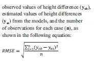
The RMSE of these models are given in table 8. RMSE for models of change in altitude vary from 3.2 cm to 4.5 cm, while RMSE for models of baseline vary between 3.1 cm and 4.5 cm.
Conclusion
This article highlights the effect of altitude change and baseline length on the differences in orthometric heights between simple geometric levelling and GPS. We have used several experimental tests on three cases of different topography.
Comparison of orthometric height differences (Hdiff) using statistical tools allows us to reach the following conclusions:
– The height difference between leveling and GPS increases very significantly with the length of baseline and depends on the topography of the terrain.
– The height difference between leveling and GPS is very significantly influenced by the altitude change.
Based on these experiments, we used linear regression to express the variation of orthometric height differences (Hdiff) as function of the baseline length, and on the altitude change for the three types of terrain. RMSE of all experimented models, vary between 3.1 cm and 4.5 cm.
At the end of these experiments, and in response to surveyors’ preoccupations, we can conclude that we could use dual frequency GPS for determining the orthometric heights, with an accuracy of a few centimeters (up to 15 cm) with respect to simple geometric levelling.
Acknowledgment
The authors would like to thank the ANCFCC for data supply used in this study.
Bibliography
ANCFCC, 2002. Situation actuelle du réseau géodésique vertical, document interne mon publie de l’ANCFCC, Mai 2002.
ANCFCC, 2012. Brochure sur le Nivellement Général Du Maroc NGM 2011, Direction de la Cartographie, Département de la Géodésie.
Battaglia, M., Segall, P., Murray, J., Cervelli, P., and Langbein, J., 2003, The mechanics of unrest at Long Valley caldera, California: 1. Modeling the geometry of the source using GPS, leveling and two-color EDM data: Journal of Volcanology and Geothermal Research, v. 127, iss. 3-4, p. 195-217.
Becker M., S. Zerbini, T. Baker, B. Bürki, J. Galanis, J. Garate, I. Georgiev, H.-G. Kahle, V. Kotzev, V. Lobazov, I. Marson, M. Negusini, B. Richter, G. Veis, and P. Yuzefovich, 2002. Assessment of height variations by GPS at Mediterranean and Black Sea coast tide gauges from the SELF projects. Global and Planetary Change, Volume 34, Issue 1, p. 5-35.
Ben Ahmed Daho S. A., 2003. Calcul des hauteurs orthométriques à partir des observations GPS : Cas d’étude : Nord de l’Algérie. 2nd FIG Regional Conference Marrakech, Morocco, December 2-5, 2003
Cakir L., Yilmaz N., 2014. Polynomials, radial basis functions and multilayer perceptron neural network methods in local geoid determination with GPS/ levelling. ScienceDirect, Measurement, Volume 57, pages 148–153.
Caporali, M., Martin S., 2000. First results from GPS measurements on present day alpine kinematics. Journal of Geodynamics, Volume 30, Issues 1–2, February 2000, Pages 275–283.
Dagnelie P. 2011. Statistique théorique et appliquée. Tome 2. Inférence statistique à une et à deux dimensions. Bruxelles, De Boeck, 736 p.
Dodson A.H., 1995. GPS for height determination, Survey Review, 33(256), pages 66–76.
Dursun Z., S., Abdullah Y. Stig-Coran M. 2002. Orthometric height derivation from GPS observations. FIG XXII International congress – Washington, D. C. USA, April 19-26 2002.
Elliott 2006. Understanding GPS principles and applications.
Guide GéoMax. Édition 2010. Guide Profiex 500. Magellan Navigation, édition 2008-2009.
Guide français ProMark 500. Magellan Navigation, édition 2008-2009.
Inside GNSS: GPS/ GALILEO/ GLONASS 2007. Weighting GNSS Observations and Variations of GNSS/ INS Integration.
Lemoine F.G., 1998. The development of the Joint NASA GSFC and NIMA Geopotential Model EGM96.
Lin, L. S., 2013. Mitigating the systematic errors of e-GPS levelling. Coordinates magazine, vol. March 2013.
Lin, L. S., 2013. Mitigating the systematic errors of e-GPS levelling. Coordinates magazine, vol. April 2013.
Norman R. Draper, Harry Smith, 1998. Applied Regression Analysis, 3rd Edition, Wiley, 736 p.
Peter J.G. 2014. Instantaneous BeiDou– GPS attitude determination: A performance analysis, Advances in Space Research, Volume 54, Issue 5, pages 851–862.
Stig-Coran M., 2002. Height Determination by GPS – Accuracy with respect to different geoid models in Sweden. FIG XXII International congress – Washington, D. C. USA, April 19-26 2002.
Xingsheng D. (2013). Transfer of height datum across seas using GPS leveling, gravimetric geoid and corrections based on a polynomial surface, Computers & Geosciences, Volume 51, pages 135–142.
Zeggai A., Benahmes Daho S.A., Ghezali B., Ayouaz A., Taibi H. et Ait Ahmes Lamara R. 2006. Conversion altimétrique des hauteurs ellipsoïdales par GPS. Article XYZ N° 109.


 (2 votes, average: 4.00 out of 5)


Leave your response!